How to grab photos from Flickr

Happy new year 2009!

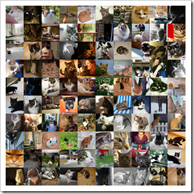
I have a post about make a Flickr image wall with Mathematica

First, you need get some basic knowledge about Flickr API, Photo Source Url

The coding is very simple, just play with it, then you can modify it to try something new.

catxml = Import[
   "http://www.flickr.com/services/rest/?method=flickr.groups.pools.getphotos&api_key=your_API_key&group_id=75601600@N00&per_page=500&page=1&safe_search=1", "XML"];

This line will do the query from Flickr group Somebody else's cat, return 500 images’ meta data

cats = Cases[catxml, XMLElement["photo", id_, {}] :> id, Infinity];
ids = #[[All, 2]] & /@ cats;
ids = RandomSample[ids, 100];

This three lines will extract 100 random photo ids

cs="http://farm"<>#[[5]]<>".static.flickr.com/"<>#[[4]]<>"/"<>#[[1]]<>"_"<>#[[3]]<>"_s.jpg" &/@ids;
imgs=Import[#] & /@ cs;

Then get the real url to each photo and import them. Here we use small size (75 by 75) “_s.jpg”

ImageAssemble[Partition[imgs, 10]]

Then put them together into one image

So we finish it just in several lines.

How to make a Ternary Plot

For the reader who are curious about the post on Ternary Plot


The code is very simple, here is the mathematica notebook, and the pdf version if the notebook somehow doesn't work.

Sorry for the late reply, I seldom check the comments for the older posts.

Tip: create 3D Map

Here is a simple explanation on how to create 3D map in the previous post.

The key is to use Extrude function (I copied it somewhere):

extrude[pts_, h_] := Module[{vb, vt, len = Length[pts], nh},
  If[! NumericQ[h], nh = 0., nh = N@h];
  vb = Table[{pts[[i, 1]], pts[[i, 2]], 0}, {i, len}];
  vt = Table[{pts[[i, 1]], pts[[i, 2]], nh}, {i, len}];
  GraphicsComplex[
   Join[vb, vt], {Polygon[Range[len]],
    Polygon[Append[
      Table[{i, i + 1, len + i + 1, len + i}, {i, len - 1}], {len, 1,
       len + 1, 2 len}]], Polygon[Range[len + 1, 2 len]]}]]

Let's create a map to show per-capita oil consumption in South America.

(* get the data *)

(* Falkland Islands is removed *)

mapdata = {First@CountryData[#, "Polygon"],
     CountryData[#, "OilConsumption"]/
      CountryData[#, "Population"]} & /@
   DeleteCases[CountryData["SouthAmerica"], "FalklandIslands"];
mapdata[[All, 2]] = Rescale[mapdata[[All, 2]]];

(* 3D map *)

Graphics3D[{EdgeForm[Darker[ColorData["Rainbow"][#[[2]]]]],
    FaceForm[ColorData["Rainbow"][#[[2]]]],
    extrude[#[[1, 1]], #[[2]]]} & /@ mapdata, Boxed -> False,
Lighting -> "Neutral", BoxRatios -> {1, 1, 0.2}, ImageSize -> 800]

The visual quality of 3D map is low, however, it is good enough for the classroom.

 

Mathematica 7: import ESRI Shape file

Finally, ESRI Shape file is supported in Mathematica 7: Import["dir/file.shp"]

However, I feel it is necessary to explain it in a little more detail for users who are not that familiar with Mathematica.

Let's import a  shape file from Indiana GIS Atlas which contains county boundaries.

(*import data*)
data=First@Import["http://129.79.145.7/arcims/statewide_mxd/downloads/LANDSURVEY_COUNTY_POLY_IN.zip", Data"];
(*check what is inside the data*)
data[[All, 1]]
{"LayerName", "Geometry", "Labels", "LabeledData"}
(* check the field name in attribute table *)
"Labels" /. data
{"AREA", "PERIMETER", "NAME_U", "NAME_L", "NCAPC"}
(* attribute data is stored in "LabeldData" *)
area = "AREA" /. ("LabeledData" /. data);
area = Rescale[area];
(* get all the geometry *)
geometry = "Geometry" /. data;
(* put two data together *)
mapdata = Transpose[{geometry, area}];
(* generate the thematic map *)
Graphics[{EdgeForm[{Thick, Gray}], FaceForm[ColorData["Rainbow"][#[[2]]]], #[[1]]} & /@ mapdata, Frame -> False, ImageSize -> 400]

 

 

With some extra efforts, a 3D version is generated.

Extract font outlines

I find this tip from the talk: Doing Physics with Mathematica 6 by Michael Trott

 

GCText[text_,tsize_]:= ImportString[ExportString[Cell[TextData[StyleBox[
text, FontWeight->"Bold",FontFamily->"Helvetica"]], "Text", tsize], "PDF"]][[1]]

outlines =  (First /@ Cases[GCText["ABC", 20], _Polygon, Infinity]);

Graphics3D[{FaceForm[],EdgeForm[Black],Polygon[Map[Append[#, 10]&, outlines, {-2}]]}];

for fun:

QHull for Mathematica

mPower.m is a Mathematica package that interfaces with qhull binaries.

Installation guide is not for windows platform.

Here is the quick way to get it running on Windows Vista with Mathematica 6.0.

1. download mPower.m, and put it into the Applications subdirectory of $UserBaseDirectory 

In[1]:= $UserBaseDirectory

Out[1]= C:\Users\...\AppData\Roaming\Mathematica

2. download qhull for windows, put it into the folder C:\qhull

3. open mPower.m, modify the following two lines,

$QHULL=ToFileName[{$UserBaseDirectory, "Applications", "qhull", "src"}]

to: $QHULL="C:\\qhull\\"

qhullFiles={"qconvex",  "qdelaunay", "qhalf","qhull", "qvoronoi"};

to: qhullFiles={"qconvex.exe",  "qdelaunay.exe", "qhalf.exe","qhull.exe", \
"qvoronoi.exe"};

4. then testing, ignore the warning on regtet and pwrvtx, we only need qhull

<< "mPower.m"

points = RandomReal[1, {10, 3}];

ch = convexHull[points, convexHullFormat -> {facetNormals -> True, facets -> True}]

 

Thanks to the mPower developers

Financial Data: AAPL vs MSFT

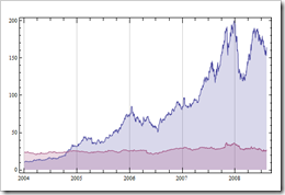
Technologically speaking, Apple and Microsoft are two quite different companies in many ways. We all know that in recently several years, Apple stock is very hot. Here is the stock price: APPL vs MSFT since 2004, the legend is not necessary for this graph.

DateListPlot[{FinancialData["AAPL",{2004}], FinancialData["MSFT",{2004}]}, Joined->True, Filling->Bottom]

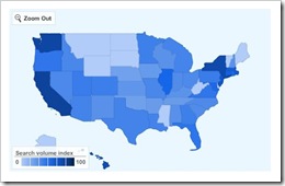
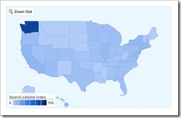
Google Insights for Search gives another way to present it.

Google search volume index for "AAPL" since 2004

Google search volume index for "MSFT" since 2004

How to extract points from a plot

pts=Cases[theplot, x_GraphicsType:>First@x, Infinity];

Example 1:

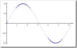
g=Plot[Sin[x],{x,0,2Pi}];
pts=Cases[g,x_Line:>First@x,Infinity];
ListPlot[pts]

Example 2:

g=Plot3D[Cos[x]+Cos[y],{x,0,4Pi},{y,0,4Pi}];
pts=Cases[g,x_GraphicsComplex:>First@x,Infinity];
ListPointPlot3D[pts]

Wolfram Screencast Gallery

There are some very impressive  presentations in Screencast Gallery.

I watched Spinthariscope by Theodore Gray. This simple shape editor is particularly interesting.

Fun with Gamepad

We have a cheap Logitech gamepad (less than 10$ from Target).

ControllerInformation[]

Controller Device 3: Logitech(R) Precision(TM) Gamepad
Raw Product Name "Logitech(R) Precision(TM) Gamepad"
Raw Product ID 49690
Device Type Windows DirectInput Device
Raw Controller Type Joystick
Mathematica Controls 22 controls
Raw Controls 12 controls

Using gamepad to rotate 3D graphics is very smooth, and can jump to top view from x, y, z directions when you hold down different buttons. It seems not supported to zoom a 3D graphic with gamepad.

Gamepad & Device Interface for the details.

Google Earth is another application to play nicely with gamepad.

Update: See here for enabling zoom function with gamepad. Thanks.

Standard Extra Packages

See here Mathematica 6.0 Standard Extra Packages

It gives out a very helpful overview on packages not loaded by default.

T-Thirt design: Pi with rainbow color scheme

Functions used: Rasterize, Grid

Something hidden

No idea? Look at the one:

Rasterize

Self random walk on sphere

Self random on sphere lattice (longitude, latitude).
(red -- starting point, green -- ending point)


Draw on a sphere:Self avoid version:

The longest horizontal lines indicate the jumps between -180 and 180.

Opacity

Nationality Name

For most counties, the nationality name usually in form of country name + suffix: -an, -ian, and -ese.
China->Chinese, Japan->Japanese, are all the east Asian the "ese" people? Let's find out with Mathematica: CountryData["Country", "NationalityName"].

From the above map, you can see it is not true at all, e.g. Korea->Korean, Thailand->Thai. Portugal->Portuguese is only "ese" country in Europe.

One thing I hear quite often is that -ese means smaller and less power as opposite to -an and -ian, -ese is used by western colonist in an insulted way. I don't know how much historic truth in this claim. Google search gives out the following:
-ian -an from Latin –ianus, meaning "native of", "relating to", or "belonging to"
-ese from the Latin -ensis, meaning "originating in"
However, it is hard to know why some countries are with "-ese", others are not.

Nonsense: Something here doesn't belong

Nonsense

Rejected logo design in the summer, 1999.

Colorful Words

Rasterize, then coloring

Minimum Bounding Rectangle of a Point Set

Give a 2-D point set, we need to find the minimum bounding rectangle in term of area.

I read it somewhere that the minimum rectangle must always contain at least one edge of the convex hull, however, I can't find a citation now. So the algorithm can be constructed in the following way: first construct the convex hull, then rotate each edges for the convex hull to the position parallel to x-axes, then calculate area of bounding rectangle; find the minimum one of these rotated rectangles and rotate it back to normal.

Nonsense

The early sign of scientist self-destruction nature.


mushroom is from http://www.wpclipart.com/plants/mushroom/mushroom.png

Google Chart API

The Google Chart API lets you dynamically generate charts.

The basic format:
http://chart.apis.google.com/chart?<parameters>

It is the most straightforward solution for web application to display dynamic graphs. I am wondering if Wolfram can come up something similar, not the webMathematica, just a simple free image generator will be great, it is definitely a good way to get more publicity.

Tips: Customizing Graphplot

For a graph g, we like draw leaves in different style from nodes.


(* find leaves *)
leaves = Complement[g[[All, 2]], g[[All, 1]]];
TreePlot[g, VertexLabeling -> False, PlotStyle -> {Black}, VertexRenderingFunction -> (If[MemberQ[leaves, #2], {FaceForm[LightGray], EdgeForm[Black], Disk[#1, 0.15], Text[#2, #1]}, {FaceForm[White], EdgeForm[Black], Disk[#1, 0.15]}] &), AspectRatio -> 0.3]

The tip is in VertexRenderingFunction, Text[#2, #1], #2 means the label, #1 is coordinates.

Learning regular expression

I am learning Regular Expression right now. Here is the example to pull the information on monthly posting activities of Mathematica Discussion Group.

url = "http://groups.google.com/group/comp.soft-sys.math.mathematica/about";
reg = "(?<=month/)\\d+-\\d+\">\\d+";
data = Import[url, "Source"];
ex = StringCases[data, RegularExpression[reg]];
ds = ToExpression[StringSplit[ex, {";", "-", "\">"}]];

Then we can use DataListPlot to produce a nice graph.

Understanding Finanical Market: Arbitrage

From Wikipedia, Arbitrage is the practice of taking advantage of a price differential between two or more markets, the profit being the difference between the markets prices.

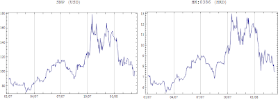
Fro example, China Petro & Chem is traded in both US and HK stock markets. The price between these two markets are different, it seems US price follows the movements of HK's in recent several months.


After converting HK share price to US dollars, the price differences can be shown:
DateListPlot[{ussnp, hksnp}, Joined -> True, Filling -> {1 -> {2}}, FillingStyle -> {Green, Red}, DateTicksFormat -> {"Month", "/", "YearShort"}]
The trick is to use Filling -> {1 -> {2}}, FillingStyle -> {Green, Red}, Green indicates HK price is higher than US price, the red means the opposite.

Tip: Orthographic view of 3D graphics

The orthographic view of the 3D plot can be generated by using ViewPoint option. It comes very handy in some situations.

data = RandomReal[1, {20, 3}];
ListPlot3D[data, InterpolationOrder -> 0, ColorFunction -> "Rainbow", Mesh -> None, Boxed -> True, Axes -> None]
Add option ViewPoint->{0,0,Infinity} and draw it again.

Then we can put together a nice bounded Voronoi diagram. It saves the trouble to use BoundedDiagram from Computational Geometry Package.

Min Max problem

There is a discussion in Matlab blog: Should min and max marry?
The question is what the overhead is in calling min and max separately, instead of scanning through the data once, looking for both the lowest and highest values, and is it worth having a combined function for min and max from a speed point of view? It seems worthy it, if you work with large data frequently.

I am not sure about how Mathematica handle Min/Max internally. The one thing I can confirm is that Min/Max operations on large random 1 dimensional array are several times faster than the ones in Matlab in my computer.

Tip on Mathematica Programming

There are two interesting presentations from 2007 Wolfram Technology Conference.

Efficient Mathematica Programming: tips from MathGroup, very helpful.
A New Mathematica Programming Style: prefix and postfix-pure function is disscussed as an alternative to the traditional matchfix-dominated style

Google Static Maps API

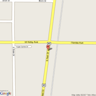
Google finally release Google Static Maps API, which allows you to generate the maps using a regular URL (ala REST) along with parameters specifying location, size, etc and it returns a unique GIF image with that map.
However, there are several drawbacks, for example, 512x512 is the largest image size allowed and geocoding is not integrated. Even though, it is better than nothing.

The following shows the API example:
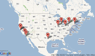
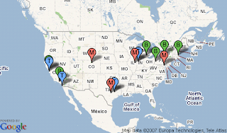
Top 10 "Mathematica" cites from Google Trends.


For fun, top 10 Mathematica cities vs top 10 Matlab cities
Red "M"--> Mathematica City, Blue "T" --> Matlab City, Green "B" --> City with both Mathematica and Matlab.


Update: static maps seems use the old data
Noticed the problem with "Trade Center Dr",
Check this place on Google Map.

Play with Images: Letter Image

Spell with Flickr is interesting. I modified the Flickr image wall code.
Here is the result:

Import High Resolution DEM (2)

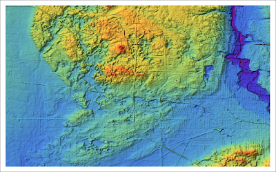
We are talking about more general case here: DEM is processed in ArcGIS (e.g. Mosaic, Extract by Mask, etc.). And it is ready for computation in Mathematica. The DEM can be exported as Float32 format, imported with the procedure in the previous post.
In this post, the DEM is exported as ARCGrid ASCII format, the whole DEM is in one text file.

data = Import["DEM.txt", {"Lines", All}];
(* the first lines are metadata *)
meta = data[[1 ;; 6]]

{"ncols 1703", "nrows 1200", "xllcorner
-86.528233463385", "yllcorner 41.430023494444", "cellsize
0.00027777777779994", "NODATA_value -9999"}

(* drop the metadata *)
data = Drop[data, 6];
(* convert string to data *)
data = Map[ToExpression, StringSplit[#]] & /@ data;

The next step is that we will make the output of ReliefPlot match the other geographic data.

1. Deal with NOData: PlotRange->{zMin,zMax}

2. Put the image into right geographic zone: DataRange-> {{Lon_Min, Lon_Max}, {Lat_Min, Lat_Max}}

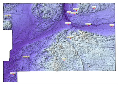
ReliefPlot[data, DataReversed->True, DataRange-> {{-86.5282, -86.0552}, {41.4300, 41.7634}}, PlotRange -> {199.0, 283.0}]

Then tested it with the map created in another post.


Note: ReliefPlot needs an option: NoData->{}

Import High Resolution DEM (1)

The best place to get high resolution DEM is from USGS National Map Seamless Server.

It publishes National Elevation Dataset (NED) in 1 arc second(~30m resolution), 1/3 arc second(~10m resolution) and 1/9 arc second(~3m resolution).

The default file format is ESRI ArcGRID. Several other non-proprietary formats are available. If you don't want to further process the DEM in ArcGIS, GridFloat format is the right choice. GridFloat is "a simple binary raster format (floating point data). There is an accompanying ASCII header file that provides file size information (number of rows and columns). The data are stored in row major order (all the data for row 1, followed by all the data for row 2, etc.)". See National Elevation Data (NED) FAQ.

Follow this tutorial for downloading procedure.

After downloading, unzip the file, .flt is the data for DEM, .hdr is the header ASCII file.

Open header file (.hdr)

ncols 650
nrows 395
xllcorner -86.428333330255
yllcorner 41.639166666159
cellsize 0.00027777777779995
NODATA_value -9999
byteorder LSBFIRST

We can see this DEM has 395 row and 650 col.

In Mathematica:

data30 = Import["ned30.flt", {"Binary", "Real32"}];
(* each row has 650 col. *)
data30 = Partition[data30, 650];
ReliefPlot[data30, DataReversed -> True, ColorFunction -> "Rainbow"]

The following examples show the same area in 1 arc second (30m) and 1/3 arc second (10m) DEMs.

30m

10m

Select Point Data inside Geographical Boundary

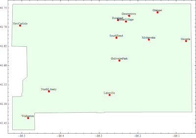
Here is an example on how to select point data inside the geographical boundary by using point inside polygon function.

(* all the cities {name, coordinates} in Indiana *)
allcities = {First[#], CityData[#, "Coordinates"]} & /@ CityData[{All, "Indiana", "UnitedStates"}];

We like to select the cities inside St. Joseph county.
Boundary of St. Joseph county is imported as Polygon. See details on importing GIS data.

In Mahtematica-users Wiki, there is an discussion on Point Inside Polygon. We choose the first solution, since it works on non-convex polygon.

(* select cities by Point inside Polygon function *)
Select[allcities, PLSPolygon[countyboundary, #[[2]]] &]

Fun with Financial Data: Currency Exchange Rates

Someone posted some interesting photos from his trip to Japan in this January. One is delicious sushi sold at the roadside in somewhere, Kyoto, Japan.


In the top row, the one marked for 900 Yen looks exactly like the ones sold here in greocery store. I am wondering the price in US dollars.

900/FinancialData["USD/JPY"] gives $8.42, it is around 60% more expensive than the ones you can get here, however, it must taste much better.

One interesting thing is how much we can get if we convert 1 USD dollar to Japan Yen through the third currency.

FinancialData[{"USD",#}] / FinancialData[{"JPY",#}] &/@ {"HKD","EUR","GBP","CAD"}
{106.842, 106.625, 106., 106.947}

Direct exchange rate is 106.825.

USD->GBP->JPY: lost near 1% USD->CAD->JPY: gain tiny 0.1%

Is there a simple way to find a currency exchange chain "USD->..->... ->JPY" to maximize the gain over "USD->JPY"?

Fun with MatrixPlot: Pixel Art

MatrixPlot is great for pixel art.

jp=MatrixPlot[pixelart, Frame->None, ColorRules->{0->White}, ColorFunction->#, ImageSize->90, Mesh->All, MeshStyle->LightGray] &/@ Append[ColorData["Gradients"], "Monochrome"]; GraphicsGrid[Partition[RandomSample[jp],8],Spacings->0]


ColorRules can be used for the better result, e.g. ColorRules -> {0 -> White, 1 -> Yellow, 2 -> Orange, 3 -> Pink, 4 -> Red}