View stock market seasonality

A reader asks about the seasonal chart. Here is a simpler version.

The seasonality is defined as the percent change from the beginning of year to the end of each month.

monthlychange[stock_, year_] :=
Module[{data, firstdateprice, endofmonthprice},
  data = FinancialData[stock, "Close", {{year, 1, 1}, {year, 12, 31}}];
  data = Map[Flatten[#] &, data]; firstdateprice = data[[1, 4]];
  endofmonthprice = Table[Last@Select[data, #[[2]] == i &][[All, 4]], {i, 12}]; (endofmonthprice/firstdateprice - 1)*100]

This will give you the monthly change of AAPL in the year of 2008.

monthlychange["AAPL", 2008]

For multiple years, the average seasonality:

mc = monthlychange["AAPL", #] & /@ Range[2000, 2008];

Mean@mc

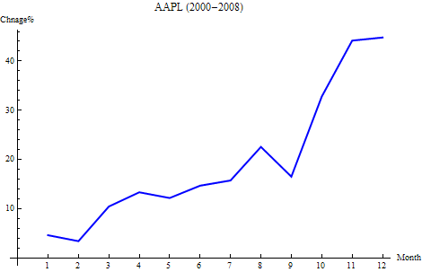
For APPL, the following graph shows the average seasonality from 2000 – 2008. According to this graph, it is probably a good idea to hold the stock through Oct and Nov before selling it.

This is a graph shows the seasonality year by year.

View stock market with heatmap

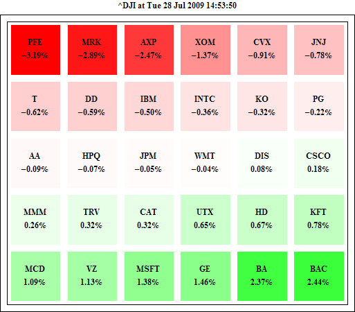
There is a heatmap tool which let you view the stock price change at a glance. It can be recreated with Mathematica in several lines of code.

Let’s pull the data by format {“symbol”, price change}

stockdata={#,(FinancialData[#]/FinancialData[#,"Close"]-1)*100 }& /@FinancialData["^DJI","Members"];

Then we need to represent the price change by color: Green means up, Red mean down, and the deeper the color, the bigger the change.

max = Max[Abs[stockdata[[All, 2]]]]; (* max change *)

GraphicsGrid[Partition[Graphics[{If[#[[2]]>=0.0,Blend[{White,Green},Rescale[#[[2]], {0,max}]], Blend[{Red,White}, Rescale[#[[2]],{-max,0}]]], Rectangle[], Black,Text[Style[#[[1]]<>"\n"<>ToString[NumberForm[#[[2]],{3,2}]]<>"%", Medium,Bold], {0.5,0.5}]}] &/@ stockdata, 6 ]]

The key function is if the price change is >0, then rescale the change in range (0, max) and get it’s color in Blend[{White, Green}]; if the price change is <0, then rescale the change in range (-max, 0) and use Blend[{Red, White}] to get the right color.

In the ascending order:

We can try other representations, too. For example, we can use the size of disk to represent the change.

Read binary file with ByteOrdering option

This is probably a very trivial problem for the ones who work on both PC and Unix platforms. I download a small DEM (478 rows by 399 columns) stored as Int16 binary from The Gloabal Land 1-km Base Elevation Project. The range of elevation is 99 ~ 397 meters.

Then in an Apple Power Mac G5:

data = BinaryReadList["mydata.bin", Table["Integer16", {399}],  478];

ArrayPlot[data, PlotRange -> {99,  397}]

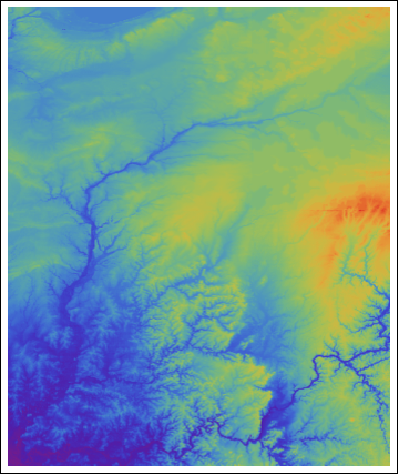
Obviously, something wrong with the numeric value loaded from the binary file. It turns out the binary is using little endian. However, the Power Mac is using big endian. You can check your system with $ByteOrdering.

Read the data again with the right ByteOrdering option.

data = BinaryReadList["mydata.bin", Table["Integer16", {399}],  478, ByteOrdering->-1];

ArrayPlot[data, ColorFunction->"Rainbow",  PlotRange -> {99,  397}]

Extract elevation data from Google Earth

In Google Earth COM API, there is a function: GetPointOnTerrainFromScreenCoords

Given an screen_x and screen_y, it returns IPointOnTerrainGE object, which gives out the {Latitude, Longitude, Altitude}

Screen coordinates range from (-1, –1) to (+1, +1)

(-1, -1) - bottom left hand corner of the screen. (0,0) - center of the screen. (1, 1) - top right hand corner of the screen.

Let’s use this function in Mathematica to extract elevation data.

First, zoom Google Earth into a testing place

Then in Mathematica:

Needs["NETLink`"]
InstallNet[]
ge = CreateCOMObject["GoogleEarth.ApplicationGE"];

getAltitude[x_, y_] :=
  Module[{pv},
   pv = ge@GetPointOnTerrainFromScreenCoords[x, y]; {pv@Longitude, pv@Latitude, pv@Altitude}];

(* extract 50 by 50 grids around the center of the screen *)
dem = Table[
   getAltitude[x, y], {x, -0.5, 0.5, 0.02}, {y, -0.5, 0.5, 0.02}];

 

 

Next situation: Given a list of {Latitude, Longitude}, how can we get the corresponding elevations for each location?

The tip is to use the camera control to move the center of screen to the given  {Latitude, Longitude}.

cam = ge@GetCamera[1];

getAltitudebyLatLon[{lat_, Lon_}] :=
Module[{pv}, cam@FocusPointLongitude = Lon;
  cam@FocusPointLatitude = lat; cam@Range = 8000; ge@SetCamera[cam, 5];
  pv = ge@GetPointOnTerrainFromScreenCoords[0, 0]; pv@Altitude]

cam@Range is the control of “eye alt”, it is in meters.

It comes very handy for extracting the cross-profile.

Control Google Earth from Mathematica

This is for Windows platform only. With Mathematica’s .NET link and Google Earth COM API, we can control Google Earth’s camera and add features directly from Matheamtica.

There is an example of planning a shortest tour through every country of the world in Document: FindShortestTour.

SC[{lat_,lon_}]:=r {Cos[lon \[Degree]] Cos[lat \[Degree]],Sin[lon \[Degree]] Cos[lat \[Degree]],Sin[lat \[Degree]]};
r=6378.7;
places=CountryData["Countries"];
centers=Map[CountryData[#,"CenterCoordinates"]&,places];
distfun[{lat1_,lon1_},{lat2_,lon2_}]:=VectorAngle[SC[{lat1,lon1}],SC[{lat2,lon2}]] r;
{dist,route}=FindShortestTour[centers,DistanceFunction->distfun];

Let’s view this example in Google Earth:

Needs["NETLink`"]
InstallNET[];

(* startup google earth *)
ge = CreateCOMObject["GoogleEarth.ApplicationGE"];

(* load path file already generated *)
ge@OpenKmlFile["d:/temp/test2.kml",1]

(* get the camera object *)
cam=ge@GetCamera[1];

(* funcion to ratate the camera *)
runcam[{lat_,lon_}]:=Module[{},
cam@FocusPointLongitude=lon;
cam@FocusPointLatitude=lat;
ge@SetCamera[cam,2]];

(* let's see the movie *)
runcam[#]&/@ centers[[route]];

Here is a low quality video.

 

Here is test2.kml for the shortest path

Here is the recorded tour (shortestrout.kmz) in Google Earth

First load test2.kml to Google Earth, then double click ShortestRoute.kmz to view the animation.