Nov 13, 2009

Make a US county thematic map using Mathematica

I read a blog entry How to Make a US County Thematic Map Using Free Tools. The idea is to use Python script to modify the style settings in SVG file to make the most recent unemployment map. Mathematica can’t import SVG file directly, however, SVG file is in XML format, it is very easy to extract the necessary data from SVG file. If you are not sure what’s going here, please refer to the original blog.

All the files are zipped together, just unzip it, run the notebook. Download it here.

usamap

Nov 2, 2009

User-defined color themes

With Blend function, it is quite simple to use user-defined color themes.

Blend[{col1, col2, col3, ...}, x]: linearly interpolates between colors coli as x varies from 0 to 1.

We like to use the following color theme:

c = {{37, 57, 175}, {40, 127, 251}, {50, 190, 255}, {106, 235,
    255}, {138, 236, 174}, {205, 255, 162}, {240, 236, 121}, {255,
    189, 87}, {255, 161, 68}, {255, 186, 133}, {255, 255, 255}};

colors = RGBColor[#/255] & /@ c;

This shows the each color in the theme:

Graphics[Table[{EdgeForm[Black], FaceForm[colors[[i]]],
   Rectangle[{i, 0}, {i + 1, 1}]}, {i, 1, Length[colors]}]]

Colordata

Check the color theme with Blend function:

DensityPlot[x, {x, 0, Length[c]}, {y, 0, 1}, AspectRatio -> Automatic,
  FrameTicks -> None, ColorFunction -> (Blend[colors, #] &),
PlotRangePadding -> None]

Colordata2

Then you probably notice how to use it in your own plot,

ColorFunction -> (Blend[colors, #] &)

Test the color theme with the data:

ReliefPlot[data, ColorFunction -> (Blend[colors, #] &)]

Colordata3

Maybe the ligher color is better.

lightercolors = Lighter[#] & /@ colors;

Colordata5

Just for fun, let’s play the color theme with an existing image.

img=ImageData[ColorConvert[place_any_image_here, ”Grayscale”]];

ArrayPlot[img, ColorFunction -> (Blend[darkercolors, #] &)]

Oct 20, 2009

Wikipedia Page Analysis

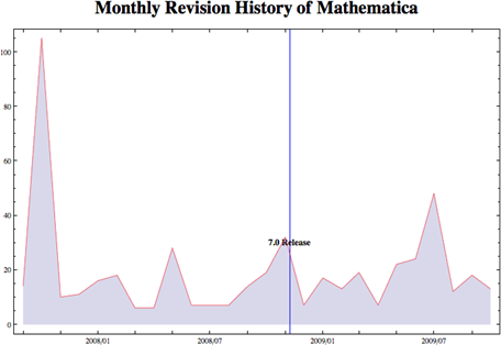
Wikipedia has lots of scientific information, however, due to its nature, it is still not considered as a research resource.  This doesn’t mean it has to be ignored. I have checked some pages related with various topics in GIS field. Most of them are well-written, the information are actually quite accurate, several contributors are the professionals in the field. In this post, I like to check some metadata information of  “Mathematica” Page on Wikipedia, it may gives us some ideas about its quality.

Tools we need: Mediawiki API and Mathematica. There are plenty examples on how to use Mediawiki api. Basic procedure is to use Import[queryurl,”XML”], then parse xml to get the information we need.

Page revision history:

(* import  contributor and timestamp *)

url = "http://en.wikipedia.org/w/api.php?action=query&prop=revisions&\
titles=Mathematica&rvprop=user|timestamp&rvlimit=500&redirects$rvuser&\
format=xml";

xml = Import[url, "XML"];
rawdata= Cases[xml, XMLElement["rev", w_, _] :> w, Infinity];
data = {"user", "timestamp"} /. rawdata;


1


2

This page is constantly revised, we probably can assume the information on “Mathematica” page is up-to-date.

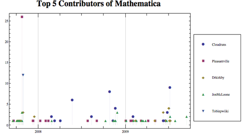
The information on the contributors is also interesting.

3 

We can dig out more information on the contributors:

(* import paged edited by each user *)

userpages[usr_] :=
  Module[{url, uxml, udata, unicase},
   url = "http://en.wikipedia.org/w/api.php?action=query&list=\
usercontribs&uclimit=500&format=xml&ucuser=" <> usr;
   uxml = Import[url, "XML"];
   udata = Cases[uxml, XMLElement["item", w_, _] :> w, Infinity];
   unicase = DeleteCases[Union["title" /. udata ],
     x_ /; (StringMatchQ[x, "User talk:" ~~ __] || StringMatchQ[x, "Talk:" ~~ __] || StringMatchQ[x, "User:" ~~ __])]; Map[usr -> # &, unicase]];


4

The common pages edited by these top5 contributors:

 5 

From the pages they have edited, they have worked on several topics closely related with Mathematica. This looks good, we may say they probably know what they are doing.

Update:

Download Wikipedia Notebook for the details.

Oct 15, 2009

Mathematica 7 on Windows 7

We just updated our machine from Windows Vista to Windows 7. I re-installed Mathematica 7 and tested with several notebooks. I didn’t notice any difference on performance.

You can re-use the license file from Vista.

C:\Users\user_name\AppData\Roaming\Mathematica\Licensing\mathpass

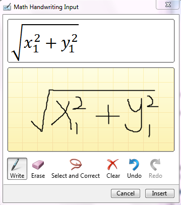
One feature I tested is Handwritten Math Recognition in Windows 7. It works very well with some simple on-screen drawings. If you use a tablet PC, this may be quite convenient in classroom.

handwriting

Sep 23, 2009

Monitor Mathematica computation with email

One of the new features in Mathematica 7.0 is allowing the sending of email directly from  any Mathematica program. It turns out very convenient for the certain situation. We have some computation tasks take long time to finish, so we  let it run on the server. The problem is that once a while I have to ssh to the server to check the outputs to make sure nothing wrong with the computation. Now with the email function, I can get the update immediately for each computation step. This is really helpful, especially now days you can check the email almost everywhere.

Picture 1

If you don’t need to check the detail, sending the update through the twitter is probably more cool.

One thing I am not sure is that how to catch the error. If there is an error raised during the computation, the math kernel can automatically send out the email with the error message, this function will be perfect.

By the way, this week I am working on an algorithm related with the Traveling Salesman Problem. If you check TSP on MathWolrd, download the notebook, you will notice it is created by a newer version of Mathematica. Open the file with any text editor, you will see:

(* CreatedBy='Mathematica 8.0' *).

Aug 25, 2009

Visualize irrational number as random walk

Irrational numbers have decimal expansions that neither terminate nor become periodic. So we can get unlimited “random walk” steps from an irrational numbers.

With the following code, the first 10000 digits of Sqrt[2] is presented as a random walk by converting it in base 4. 0, 1, 2 and 3 digit in base 4 represent 4 directions. Starting point is the green dot, the red one is the ending point.

x = N[Sqrt[2], 10000];
walk = First@ RealDigits[x, 4];
rn = FoldList[Plus, {0, 0}, {{0, 1}, {1, 0}, {0, -1}, {-1, 0}}[[# + 1]] & /@ walk];
Graphics[{Line[rn], PointSize[Large], Green, Point[First@rn], Red, Point[Last@rn]}]

randomwalk1

We can also display it with ArrayPlot by constructing a sparse array.

(* shift the moves to {1,1} *)

minx = Min[rn[[All, 1]]];
miny = Min[rn[[All, 2]]];
m = # + {-minx + 1, -miny + 1} & /@ rn;

(* sparse array *)

tt = Tally[m];
cd = SparseArray[tt[[All, 1]] -> tt[[All, 2]]];
cd = Transpose[cd];
ArrayPlot[cd, ColorFunction -> "Rainbow", DataReversed -> True, ColorRules -> {0 -> White}]

randomwalk2

Let’s visualize Sqrt[2], e, Pi in their first 50000 digits. It seems there are some similarities among these images.

Sqrt[2]

2

Pi

Pi

e

e

Update:

DrMajorBob said... in comments:

Here's a 3D version:

x = N[Sqrt[2], 10000];
walk = First@RealDigits[x, 6];
rn = FoldList[ Plus, {0, 0, 0}, {{0, 1, 0}, {1, 0, 0}, {0, -1, 0}, {-1, 0, 0}, {0, 0, 1}, {0, 0, -1}}[[# + 1]] & /@ walk ];
Graphics3D[{Line[rn], PointSize[Large], Green, Point[First@rn], Red, Point[Last@rn]}]


3d

You can also try non-irrational number, e.g. 121/5^10

Thanks.

Update 2:

Visualize genome sequence. I know nothing about it, it probably totally meaningless.

GenePlot[g_] := Module[{cs, rn}, walk = Characters[GenomeData [g, "FullSequence"]] /. {"A" -> 1,  "T" -> 2, "G" -> 3, "C" -> 4};
  rn = FoldList[Plus, {0, 0}, {{0, 1}, {1, 0}, {0, -1}, {-1, 0}}[[#]] & /@ walk];
  Graphics[{Line[rn], PointSize[Large], Green, Point[First@rn], Red, Point[Last@rn]}, Frame -> True, FrameTicks -> None] ]

GenePlot["DDK4"]

geneplot

GenePlot["DKK3"]

geneplot2

Aug 12, 2009

Display a plot by clicking a button

Ok, this seems to be very easy in Mathematica.

Button["Show me a plot", Show[Plot[Sin[x], {x, -Pi, Pi}]]]

Then you click the button, nothing happens.

Button["Show me a plot", Print[Plot[Sin[x], {x, -Pi, Pi}]]]

This line will do the job. Or use the following line:

Show[Plot[Sin[x], {x, -Pi, Pi}],
DisplayFunction -> (Button["Show me a plot", Print[#]] &)]

The key here is to use “Print” rather than “Show”. It isn’t clearly explained in the “ref/Button”.

Aug 7, 2009

View weighted graph with GraphPlot

Here is a simple example on how to customizing Graphplot. We like to use GraphPlot to visualize the number of people who commute into or out Monroe county from/to its neighbor counties.

g={{"Owen" -> "Monroe", 2813}, {"Greene" -> "Monroe",
  3788}, {"Lawrence" -> "Monroe", 4022}, {"Jackson" -> "Monroe",
  85}, {"Brown" -> "Monroe", 689}, {"Morgan" -> "Monroe",
  821}, {"Monroe" -> "Owen", 676}, {"Monroe" -> "Greene",
  207}, {"Monroe" -> "Lawrence", 679}, {"Monroe" -> "Brown",
  303}, {"Monroe" -> "Morgan", 617}}

vercoor={"Monroe" -> {-86.529, 39.1621}, "Owen" -> {-86.7642, 39.2868}, "Greene" -> {-86.9403, 39.0246},  "Lawrence" –> {  -86.4923,  38.8627}, "Jackson" -> {-86.0462, 38.8798},  "Brown" -> {-86.2382, 39.203}, "Morgan" -> {-86.4238, 39.4233}}

First try:

GraphPlot[g, VertexLabeling -> True, VertexCoordinateRules -> vercoor]

graphplot1

Using arrow to indicate in/out seems to be a good idea. We use EdgeRenderingFunction in second try:

GraphPlot[g, VertexLabeling -> True,
EdgeRenderingFunction -> (Arrow[#1, 0.05] &),
VertexCoordinateRules -> vercoor]

graphplot2

However, the labels on the edge is lost. We can handle it in EdgeRenderingFunction.

GraphPlot[g, VertexLabeling -> True,
EdgeRenderingFunction -> ({Text[#3, Mean[#1]], Arrow[#1, 0.05]} &),  VertexCoordinateRules -> vercoor]

graphplot3

The graph is still difficult to read, the commuting pattern isn’t clear at a glance. We further update EdgeRenderingFunction and use the line color and thickness to show the pattern.

GraphPlot[g,
EdgeRenderingFunction -> ({If[#2[[1]] == "Monroe", Red, Blue],
     AbsoluteThickness[0.5 + #3/500], Arrowheads[0.02 + #3/120000],  Arrow[#1, 0.05]} &), VertexLabeling -> True,
VertexCoordinateRules -> vercoor]

graphplot4

In the last try, we use VertexRenderingFunction to make the label more clear.

GraphPlot[g,
EdgeRenderingFunction -> ({If[#2[[1]] == "Monroe", Red, Blue],
     AbsoluteThickness[0.5 + #3/500], Arrowheads[0.02 + #3/120000], Arrow[#1, 0.06]} &), VertexLabeling -> True,
VertexCoordinateRules -> vercoor,
VertexRenderingFunction -> ({Text[Style[#2, 14, Bold], #2 /. vercoor, Background -> White]} &)]

graphplot5

Import the shapefile, then you get a map:

graphplot6

Jul 29, 2009

View stock market seasonality

A reader asks about the seasonal chart. Here is a simpler version.

The seasonality is defined as the percent change from the beginning of year to the end of each month.

monthlychange[stock_, year_] :=
Module[{data, firstdateprice, endofmonthprice},
  data = FinancialData[stock, "Close", {{year, 1, 1}, {year, 12, 31}}];
  data = Map[Flatten[#] &, data]; firstdateprice = data[[1, 4]];
  endofmonthprice = Table[Last@Select[data, #[[2]] == i &][[All, 4]], {i, 12}]; (endofmonthprice/firstdateprice - 1)*100]

This will give you the monthly change of AAPL in the year of 2008.

monthlychange["AAPL", 2008]

For multiple years, the average seasonality:

mc = monthlychange["AAPL", #] & /@ Range[2000, 2008];

Mean@mc

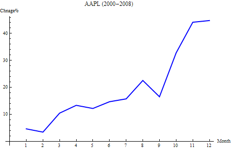
For APPL, the following graph shows the average seasonality from 2000 – 2008. According to this graph, it is probably a good idea to hold the stock through Oct and Nov before selling it.

seasonality

This is a graph shows the seasonality year by year.

seasonality2

Jul 28, 2009

View stock market with heatmap

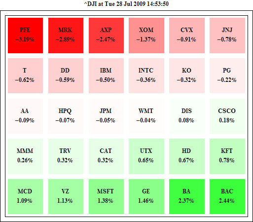
There is a heatmap tool which let you view the stock price change at a glance. It can be recreated with Mathematica in several lines of code.

Let’s pull the data by format {“symbol”, price change}

stockdata={#,(FinancialData[#]/FinancialData[#,"Close"]-1)*100 }& /@FinancialData["^DJI","Members"];

Then we need to represent the price change by color: Green means up, Red mean down, and the deeper the color, the bigger the change.

max = Max[Abs[stockdata[[All, 2]]]]; (* max change *)

GraphicsGrid[Partition[Graphics[{If[#[[2]]>=0.0,Blend[{White,Green},Rescale[#[[2]], {0,max}]], Blend[{Red,White}, Rescale[#[[2]],{-max,0}]]], Rectangle[], Black,Text[Style[#[[1]]<>"\n"<>ToString[NumberForm[#[[2]],{3,2}]]<>"%", Medium,Bold], {0.5,0.5}]}] &/@ stockdata, 6 ]]

The key function is if the price change is >0, then rescale the change in range (0, max) and get it’s color in Blend[{White, Green}]; if the price change is <0, then rescale the change in range (-max, 0) and use Blend[{Red, White}] to get the right color.

HeatMap1

In the ascending order:

HeatMap2

We can try other representations, too. For example, we can use the size of disk to represent the change.

HeatMap3

Jul 16, 2009

Read binary file with ByteOrdering option

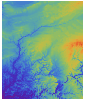
This is probably a very trivial problem for the ones who work on both PC and Unix platforms. I download a small DEM (478 rows by 399 columns) stored as Int16 binary from The Gloabal Land 1-km Base Elevation Project. The range of elevation is 99 ~ 397 meters.

Then in an Apple Power Mac G5:

data = BinaryReadList["mydata.bin", Table["Integer16", {399}],  478];

ArrayPlot[data, PlotRange -> {99,  397}]

dem2

Obviously, something wrong with the numeric value loaded from the binary file. It turns out the binary is using little endian. However, the Power Mac is using big endian. You can check your system with $ByteOrdering.

Read the data again with the right ByteOrdering option.

data = BinaryReadList["mydata.bin", Table["Integer16", {399}],  478, ByteOrdering->-1];

ArrayPlot[data, ColorFunction->"Rainbow",  PlotRange -> {99,  397}]

dem1

Jul 9, 2009

Extract elevation data from Google Earth

In Google Earth COM API, there is a function: GetPointOnTerrainFromScreenCoords

Given an screen_x and screen_y, it returns IPointOnTerrainGE object, which gives out the {Latitude, Longitude, Altitude}

Screen coordinates range from (-1, –1) to (+1, +1)

(-1, -1) - bottom left hand corner of the screen. (0,0) - center of the screen. (1, 1) - top right hand corner of the screen.

Let’s use this function in Mathematica to extract elevation data.

First, zoom Google Earth into a testing place

googleearth

Then in Mathematica:

Needs["NETLink`"]
InstallNet[]
ge = CreateCOMObject["GoogleEarth.ApplicationGE"];

getAltitude[x_, y_] :=
  Module[{pv},
   pv = ge@GetPointOnTerrainFromScreenCoords[x, y]; {pv@Longitude, pv@Latitude, pv@Altitude}];

(* extract 50 by 50 grids around the center of the screen *)
dem = Table[
   getAltitude[x, y], {x, -0.5, 0.5, 0.02}, {y, -0.5, 0.5, 0.02}];


dem 

Next situation: Given a list of {Latitude, Longitude}, how can we get the corresponding elevations for each location?

The tip is to use the camera control to move the center of screen to the given  {Latitude, Longitude}.

cam = ge@GetCamera[1];

getAltitudebyLatLon[{lat_, Lon_}] :=
Module[{pv}, cam@FocusPointLongitude = Lon;
  cam@FocusPointLatitude = lat; cam@Range = 8000; ge@SetCamera[cam, 5];
  pv = ge@GetPointOnTerrainFromScreenCoords[0, 0]; pv@Altitude]

cam@Range is the control of “eye alt”, it is in meters.

It comes very handy for extracting the cross-profile.

GoolgeEarth2

Jun 19, 2009

Control Google Earth from Mathematica

This is for Windows platform only. With Mathematica’s .NET link and Google Earth COM API, we can control Google Earth’s camera and add features directly from Matheamtica.

There is an example of planning a shortest tour through every country of the world in Document: FindShortestTour.

SC[{lat_,lon_}]:=r {Cos[lon \[Degree]] Cos[lat \[Degree]],Sin[lon \[Degree]] Cos[lat \[Degree]],Sin[lat \[Degree]]};
r=6378.7;
places=CountryData["Countries"];
centers=Map[CountryData[#,"CenterCoordinates"]&,places];
distfun[{lat1_,lon1_},{lat2_,lon2_}]:=VectorAngle[SC[{lat1,lon1}],SC[{lat2,lon2}]] r;
{dist,route}=FindShortestTour[centers,DistanceFunction->distfun];

Let’s view this example in Google Earth:

Needs["NETLink`"]
InstallNET[];

(* startup google earth *)
ge = CreateCOMObject["GoogleEarth.ApplicationGE"];

(* load path file already generated *)
ge@OpenKmlFile["d:/temp/test2.kml",1]

(* get the camera object *)
cam=ge@GetCamera[1];

(* funcion to ratate the camera *)
runcam[{lat_,lon_}]:=Module[{},
cam@FocusPointLongitude=lon;
cam@FocusPointLatitude=lat;
ge@SetCamera[cam,2]];

(* let's see the movie *)
runcam[#]&/@ centers[[route]];

Here is a low quality video.


Here is test2.kml for the shortest path

Here is the recorded tour (shortestrout.kmz) in Google Earth

First load test2.kml to Google Earth, then double click ShortestRoute.kmz to view the animation.

Jun 17, 2009

Mathematica 7: Export ESRI shapefile

One way to achieve this goal is by using the spatial database. Oracle and PostgreSQL have excellent supports of spatial data types. All you need to do is to connect the database in Mathematica and insert the data into the spatial database. There are tools come with databases allow you to dump the data into a shapefile. If you need a light-weighted spatial database, you can try SpatiaLite, it is based on popular SQLite.

For Windows platform, download the followings first:

spatialite-tools and init_spatialite-2.3.sql

upzip them and copy spatialite.exe and init_spatialite-2.3.sql into the same folder.

In this example, we like to export the following information to a shape file:

data={First[#], CityData[#,"Population"], CityData[#,"Longitude"], CityData[#,"Latitude"]} &/@ CityData [{All, "Indiana", "UnitedStates"}];

We need write some SQLs:

CREATE TABLE Towns (Name TEXT, Population INTEGER);
SELECT AddGeometryColumn('Towns','LonLat', 4326,'Point',2);

4326 means  EPSG 4326, the coordinate reference system of WGS84(longitude, latitude) pair coordinates in degrees.

To Insert the data:

INSERT INTO Towns (Name, Population, LonLat) Values ('Indianapolis', 784118, GeomFromText ('Point(-86.1477 39.7909)', 4326));

In Mathematica, this will create all the “INSERT” statements

str="INSERT INTO Towns (Name, Population, LonLat) Values ('v1', v2, GeomFromText('Point(v3 v4)',4326));"

strs=StringReplace[str, {"v1"->#[[1]], "v2"->ToString[#[[2]]],"v3"->ToString[#[[3]]], "v4"->ToString[#[[4]]]}] &/@ data;

Export["insert.txt", strs]

Then we can put all the SQL statements together into one file (test.sql):

BEGIN;
CREATE TABLE Towns (Name TEXT, Population INTEGER);
SELECT AddGeometryColumn('Towns','LonLat', 4326,'Point',2);
… INSERT INTO commands is here …
COMMIT;

In window command line mode:

spatialite.exe -init init_spatialite-2.3.sql test.sqlite < test.sql

So far, we have got all the data from Mathematica into the table Towns in test.sqlite.

run: spatialite.exe test.sqlite, and check if the records inside are right, then dump the shapefile:

.dump Towns LonLat towns_shp ASCII POINT;

Import the town_shp.shp back into Mathametica:

Show[Import["towns_shp.shp"], Frame -> True, FrameTicks -> Automatic]

towns

More information: SpatiaLite Tutorial

If you are not comfortable with command-line tools, there is a GUI tool for SpatiaLite.

Mar 24, 2009

Testing the new map with Mathematica

Generally speaking, when dealing with GIS data, you probably shouldn’t put Mathematica in top of your list.  However, when you want to develop a new algorithm or visualization, Mathamtica is a good choice to test the prototype.

Here is an example:

newmap01  

The same map in the “forest” looking.

newmap2

Mar 7, 2009

Tip: processing large data sets

When deal with large data sets, ReadList is more efficient than Import.

From documentation:

If file is not already open for reading, ReadList opens it, then closes it when it is finished. If the file is already open, ReadList does not close it at the end.

ReadList[stream] reads from an open input stream, as returned by OpenRead.

So we can use OpenRead to open the file, then use ReadList to load large data sets piece by piece.

str = OpenRead[datafile]

(* the first number in our data file is the total number of points *)

ReadList[str, Number, 1]

{17581099}

Then we can read the real data in much smaller pieces every time, otherwise it may not have enough memory to run the processing algorithm.

Here is the example

(* read first 5 records *)

ReadList[str, Number, 7*5, RecordLists -> True] // MatrixForm

data1

(* read the next 5 records *)

ReadList[str, Number, 7*5, RecordLists -> True] // MatrixForm

data2

At the end, close the file by

Close[str]

Feb 27, 2009

Antialiasing in 3D graphics

From documentation, this is a new feature in Mathematica 7.0:

“For 3D graphics, the operation of Antialiasing can depend on the particular graphics hardware you are using. Antialiasing is disabled unless Allow Antialiasing is set in the Preferences dialog.”

2

See the difference:

3

If you use a laptop with the integrated on-board  video, antialiasing in 3D may not be supported at all.

Feb 22, 2009

Counting coins with image processing

Today I read a paper about automatically counting trees from satellite image, that makes me remember the coin-counting example from image processing class which I took many years ago.

I put some coins on the back of the mouse pad, snap a photo with the web camera.

picanom-picture-01-2009-02-22

img2 = Binarize[img]

countcoin2

img3 = ArrayPlot[MorphologicalComponents[img2]]

countcoin3

Now let’s do the counting.

cd = Tally[Flatten[MorphologicalComponents[img2]]]

{{0, 162643}, {1, 7600}, {2, 7633}, {3, 7369}, {4, 4309}, {5,
  7679}, {6, 5868}, {7, 5883}, {8, 4082}}

(* pick the image region which is possible for the coins *)

cd2 = Select[cd[[All, 2]], # > 500 && # < 10000 &]

ListPlot[cd2, PlotStyle -> {PointSize[Large]}]

countcoin4

Clearly, there are three different groups of coins

Total[Map[Length, Sort[FindClusters[cd2]]] {5, 10, 25}]

130

Using $xxxx Mathematica to counting coins is kind of stupid itself, however, there are plenty of engineering applications actually do the very similar things in more complex situations.