Feb 27, 2009

Antialiasing in 3D graphics

From documentation, this is a new feature in Mathematica 7.0:

“For 3D graphics, the operation of Antialiasing can depend on the particular graphics hardware you are using. Antialiasing is disabled unless Allow Antialiasing is set in the Preferences dialog.”

2

See the difference:

3

If you use a laptop with the integrated on-board  video, antialiasing in 3D may not be supported at all.

Feb 22, 2009

Counting coins with image processing

Today I read a paper about automatically counting trees from satellite image, that makes me remember the coin-counting example from image processing class which I took many years ago.

I put some coins on the back of the mouse pad, snap a photo with the web camera.

picanom-picture-01-2009-02-22

img2 = Binarize[img]

countcoin2

img3 = ArrayPlot[MorphologicalComponents[img2]]

countcoin3

Now let’s do the counting.

cd = Tally[Flatten[MorphologicalComponents[img2]]]

{{0, 162643}, {1, 7600}, {2, 7633}, {3, 7369}, {4, 4309}, {5,
  7679}, {6, 5868}, {7, 5883}, {8, 4082}}

(* pick the image region which is possible for the coins *)

cd2 = Select[cd[[All, 2]], # > 500 && # < 10000 &]

ListPlot[cd2, PlotStyle -> {PointSize[Large]}]

countcoin4

Clearly, there are three different groups of coins

Total[Map[Length, Sort[FindClusters[cd2]]] {5, 10, 25}]

130

Using $xxxx Mathematica to counting coins is kind of stupid itself, however, there are plenty of engineering applications actually do the very similar things in more complex situations. 

Feb 16, 2009

Howto: Display 2D plot in 3D

In GIS field, sometimes we like to stack several 2D plots together and display them inside a 3D box. For Mathematica, we need to define a function to convert a 2D plot into a 3D graphic object. I will use a small Geotiff as an example, you can download it here if you like to try the code.

(*get the ElevationRange, then import data *)

Import["smalldem.tif", {"Geotiff", "ElevationRange"}]

data = Import["smalldem.tif", {"Geotiff", "Data"}];

Then we a create the contour plot with 100 feet contours

c1=ListContourPlot[data,MaxPlotPoints->30,Contours->Function[Range[650,850,100]],ColorFunction->”DarkTerrain”,PlotRange->{640,850}]

Here the function we need to convert 2D plot into 3D

to3d[plot_,height_,opacity_]:=Module[{newplot}, newplot = First@Graphics[plot];newplot=N@newplot /. {x_?AtomQ,y_?AtomQ}->{x,y, height} ;
newplot /. GraphicsComplex[xx__]->{Opacity[opacity], GraphicsComplex[xx]}];

This function has three parameters: 2D plot, height, and opacity

Let’s create two more contour plots with 50 and 20 feet contours respectively. Then we can stack them together by setting them in different heights.

Show[{Graphics3D[to3d[c1,30,0.75]]}, Graphics3D[to3d[c2,20,0.75]], Graphics3D[to3d[c3,10,0.75]], Lighting->"Neutral", BoxRatios->{1,1,0.8},Axes->True]

listcontourplot02

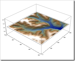
Then we like to stack the original geotiff at the very bottom. This time we need to convert the raster into 3D. I use the example you can find in Listplot3D (check the section of “Neat Examples”).

r1=ReliefPlot[data,ColorFunction->colorf,ImagePadding->None, Frame->False, ImageSize->{800,800}];

pic = Reverse[ImageData[r1]];

bg=ListPlot3D[Table[1,{x,1,800,5},{y,1,800,5}],Mesh->None, VertexColors->{pic[[1;;800;;5,1;;800;;5]]},DataRange->{{1,800},{1,800}}, Lighting->"Neutral"]
listcontourplot03

The final product:

listcontourplot01

Here is the complete notebook.

Feb 13, 2009

Display large DEM with MaxPlotPoints

MaxPlotPoints is a very useful option when works with large DEM.

dem=Import[tif,{"GeoTIFF","Data"}];
Dimensions[dem]
{2825, 5075}

Try ReliefPlot[dem], it takes a very long processing time in my not-up-to-date computer, on the other hand, with limited monitor resolutions, it doesn’t make sense to draw every point of this DEM.

Let’s first try:

ReliefPlot[dem, MaxPlotPoints –> 25]

 dem01

Not quite good, the pixel is in rectangle shape rather than square, then with the small adjustment:

ReliefPlot[dem, MaxPlotPoints -> {50, 25}]

 dem02

ReliefPlot[dem, MaxPlotPoints -> {1000, 500},
ColorFunction -> "GreenBrownTerrain"]

Click to see the large image, please ignore the left part, it is a quality issue from the DEM data source.

dem05

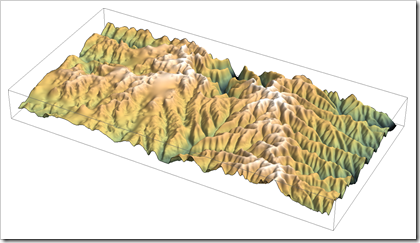
The same rule goes with ListPlot3D, if you want to get a 3D version.

ListPlot3D[dem, MaxPlotPoints -> {600, 300}, Mesh -> None,
Axes -> None, ColorFunction -> "GreenBrownTerrain",
BoxRatios -> {2, 1, 0.2}, ImageSize -> 1200]

idem06

Feb 11, 2009

Import water data from National Weather Service

Besides real-time water data from USGS in the previous post, we like to import more data from National Weather Service, it has the forecast data on water stage.

The data is distributed in XML format.

NWSxml=Import[http://www.crh.noaa.gov/ahps2/xml/nori3_hgirg.xml];

(* function to extract data from xml *)

extractdata[xml_,group_]:=Module[{dataxml,groupdata},dataxml=Cases[NWSxml,XMLElement[group,_,_],Infinity];
groupdata=Transpose[Cases[dataxml,XMLElement["datum",{},{___,XMLElement[#,_,{x_}],___}]:>x,Infinity]&/@{"valid","primary","secondary"}];
groupdata /. {x_,y_,z_}:> {StringReplace[StringDrop[x,-9],{"T"->" "}],ToExpression[y],ToExpression[z]*1000}];

(* extract data*)

observeddata = extractdata[NWSxml, "observed"];
forecastdata = extractdata[NWSxml, "forecast"];

(* produce the graph *)

importNWSxml

Flood stage is at 11.0 feet, it seems the white river may be in the flood stage in next several days.

Feb 10, 2009

Import USGS national real-time water data

The built-in real-time weather data in Mathematica 7.0 is wonderful. You may be interested in importing more related data.

USGS has web-interface for Daily Streamflow Conditions

Here is the simple steps from importing Gauge height and Discharge data

USGS 03353800 White Lick Creek at Mooresville, IN

(*import html as plain text *)

rawdata=Import[“http://waterdata.usgs.gov/nwis/uv?cb_00060=on&cb_00065=on&format=html&period=7&site_no=03353800”];

(* extract table information *)

rawdata=StringReplace[rawdata,","->""];
result=StringCases[rawdata,x:DatePattern[{"Month","/","Day","/","Year"," ","Hour",":","Minute"}]~~Whitespace~~y:NumberString~~Whitespace~~z:NumberString:>{x,ToExpression[y],ToExpression[z]}];

(*draw graph*)

DateListPlot[result[[All,1;;2]],PlotStyle->{Blue, PointSize[Medium]},PlotLabel->"Site: 03353800",Joined->True,Filling->Bottom,FrameLabel->{"Time","Gage Height (feet)"},DateFunction:>(DateList[{#,{"Month","/","Day","/","Year"," ","Hour",":","Minute"}}]&),DateTicksFormat->{"MonthShort","/","Day"," ","Hour",":","Minute"}]

By the way, the code is tested in Mathematica 6.0.