Tip: Import 3D Model

For whatever reason, some 3D models have to be imported in Mathematica.
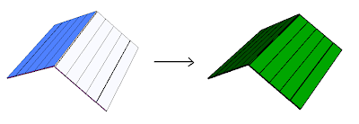
The 3D model is stored as OBJ file. When it is imported, it loses the texture information.

(* set the color *)
roof = Import["greenroof.obj"]
roof = roof /. {l_Line :> {Thick,Black, l}, p_Polygon :> {FaceForm[Darker[Green]], p}}

Here the whole model:

Tip: Mathematica version of Maltab "Find" Function

I must say that if you work with Matlab everyday, it is really frustrated with Mathematica in some points.

Find is one of the most frequently used functions in Matlab.
Find(array>5.0): returns indices of the elements that are greater than 5.0.

In Mathematica, the corresponding function is Position

Position[array, #>5.0&] or Position[array, _>5.0] just doesn't work.

We "simple-minded" Matlab user have seldom thought about putting constraints on patterns

Then, this will do the job

Position[array, x : _ /; x > 5.0]

Position[array, x:_ /; testfunc[x]] will do better.

Tip: ListPlot3D and InterpolationOrder

Not exactly a tip.

10,000 random points
Regular grid: data = Table[RandomReal[], {100}, {100}];
Irregular grid: data = RandomReal[1, {10000, 3}];

Table[ListPlot3D[data, InterpolationOrder -> n, Mesh -> None]; // Timing, {n, {0, 1, 2, 3, 4}}]

Result (in seconds):
Interplotion Order: 0, 1, 2, 3, 4
Regular Gird: 0.771, 3.415, 3.435, 3.525, 3.565
Irregular Grid:6.349, 4.871, 4.767, 4.777, 4.737

Difference in zero-order interpolation is huge.

Reference: InterpolationOrder

Tip: Counting Files by Date

We like to know the number of the certain special type file processed month by month.
The following code will do the job:

(* all the files under one base direcotry *)
SetDirectory[basedirectory]
(* find all the files in all the subdirectories*)
files = FileNames["*.byt", {"*"}, Infinity];
(* return {year, month} for each file *)
data = Take[FileDate[basedirectory <> "\\" <> #], 2] & /@ files;
(* sort then count *)
cs = Tally[Sort[data]];
(* draw the graph *)
DateListPlot[cs, Filling -> Bottom, FillingStyle -> Blue, PlotStyle -> {Red, PointSize[Large]}, PlotRange -> {{{2006, 1}, {2008, 2}}, Automatic}, DateTicksFormat -> {"MonthShort", "/", "YearShort"}]

Fun with Map: Simple Geocoding with Yahoo Map API

Yahoo Map API has a simple REST interface which works well with Mathematica.
Here is an example to show a simple Geocoding function.

Problem: Give an address, return (longitude, latitude)

The basic query format:
http://local.yahooapis.com/MapsService/V1/geocode?appid=YahooDemo
&street=?&city=?&state=?


Let's try it with the address of Wolfram Research Inc.

geocoding[{"100 Trade Center Drive", "Champaign", "IL"}]
{-88.244868, 40.097855}

Is the result right? Let's check it out with Map Image API.


image[geocoding[{"100 Trade Center Drive", "Champaign", "IL"}]]



Notice:
1. I use "YahooDemo" as AppID, if you want to use this function frequently, please apply your own ID, it is free.
2. The Geocoding API is limited to 5, 000 queries per IP per day, Google Map has the similar limitation, so if you need geocoding a large amount of addresses, please use offline geocoding application.

reference: Yahoo Map API, Map Image API, Geocoding API

update:
Google version: see 1th comment , Thanks very much.

Tip: Programming Style

Read it from the company newsletter sometime ago:

Given a list of pairs of numbers, return a list consisting of the sum of each pair.
pairs = {{58, 96}, {85, 22}, {100, 69}, {5, 37}, {32, 64}, {41, 86}, {14, 0}, {79, 22}, {55, 36}, {86, 39}, {11, 15}};

(* Style I*)
result = Table[Null, {Length[pairs]}];
Do[result[[k]] = pairs[[k, 1]] + pairs[[k, 2]], {k, 1, Length[pairs]}]
result
(* Style II *)
Table[pairs[[k, 1]] + pairs[[k, 2]], {k, Length[pairs]}]
(* Style III *)
Apply[Plus, pairs, {1}]
(* Style IV *)
Map[Total, pairs]
(* Style V *)
pairs /. {p_, q_} -> p + q
(* Style VI *)
pairs[[All, 1]] + pairs[[All, 2]]

I work with Maltab most of the time, it is useful to read this kind of document occasionally.

Details on Importing GIS Data

If you live US, there are plenty of GIS data published by different government agencies, it is quite possible that the county where you live has its own GIS department now. Most of the vector data come in ESRI shape file format. There are several different ways to get shape file into Mathematica. One simple way is explained here, it uses tools based on shapelib (open source tools to read/write shape file).

Step 1. Find the data you want
Just go to the agency may have the data you are interested. In this example, I will use the Indiana county boundary data I have.
There are some free/open source GIS software you can use to check the data: Quantum GIS, ArcGIS Explorer. (No offense here, I just assume you don't much about GIS.)

Step 2. Output shaple file to data
We use shp2text, and you can find more information on its website.
In command line mode:
shp2text --gpx indiana.shp
the output is the structure of the associated data in DBF file. We like to have county name, it is in Field 1.
Field 0: Type=Integer, Title=`FIPS', Width=5, Decimals=0
Field 1: Type=String, Title=`COUNTY', Width=16, Decimals=0
Field 2: Type=String, Title=`DOQ_DISK', Width=16, Decimals=0
Field 3: Type=String, Title=`FIPS_STRG', Width=16, Decimals=0
Field 4: Type=String, Title=`ATLAS_CODE', Width=16, Decimals=0
Field 5: Type=Double, Title=`AREA_FT2', Width=19, Decimals=3
Field 6: Type=Double, Title=`AREA_ACRES', Width=19, Decimals=3
Field 7: Type=Double, Title=`PERIMETER_', Width=19, Decimals=3

shp2text --gpx indiana.shp 1 0 > output.xml

There will dump the shape file into xml file, of course, if you can dump it into plain text without "--gpx", and reformat the plain text to cvs format. I personally prefer to XML format.


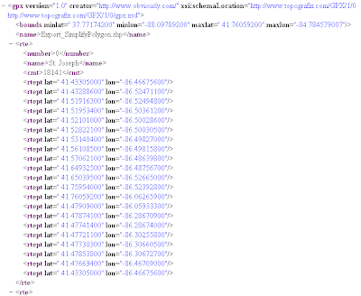
see the whole document here.

Step 3. Process XML file in Mathematica
I listed the code step by step here in case you are not familiar with XML.

dataxml = Import["output.xml"];
(* extract county names *)
countyname = Drop[Cases[dataxml, XMLElement["name", __, {w_}] :> w, Infinity], 1];
(* extract {lat, lon} for each county boundary *)
wholes=Cases[dataxml, XMLElement["rte", __], Infinity] ;
counties = (Cases[#, XMLElement["rtept", __], Infinity] & ) /@ wholes;
dataLatLon = counties /. (XMLElement["rtept", latLonRules_, {}] :> { {"lat", "lon"} /. latLonRules });
(* tidy up a little, of course, you can combine them into one line code*)
test = Flatten[#, 1] & /@ dataLatLon;
test = Map[ToExpression, test];
test = Map[Reverse, test, 2];
(* then draw it *)
Graphics[{EdgeForm[Gray], FaceForm[LightGreen], Polygon[test]}]

Here is the example that uses the data imported as the background map.
Point data is from CityData, and it shows all cities with population > 1000.


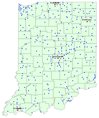
Importing point, line type of data is in the similar way.

Tip: Efficient Plot Large Point Data Set

It is from the discussion from math group.
Point, Line and Polygon now accept multi-coordinate list that can be processed and rendered more quickly by the Mathematica front end than the equivalent individual primitives.

data = Table[{Random[], Random[]}, {100000}];
Graphics[{PointSize[0.002], Point[data]}, AspectRatio -> Automatic]
Graphics[{PointSize[0.002], Point[#] & /@ data}, AspectRatio -> Automatic]

More information: Efficient Representation of Many Primitives

Old Time Fun: Ternary Plot

Here is the ternary plot of the 140 named colors supported by modern browsers. Actually, only 139 colors are drawn in the graph. There is no place for Black (RGBColor[0,0,0]), the center is White, however, you can't see it on the white background.

Old Time Fun: Binary Image

Can you find out the relationship between these two images?

Old Time Fun: Hilbert Curve

At the time I started learning Mathematica (maybe version 3.0), it is almost impossible for any student not to plot space filling curves or other fancy fractals. Except for eye candy, it is quite useless for most of us. Today, it can't even be counted as eye candy any more.
Here is mine, Hilbert Space Filling Curve, which I found in pile of old files, the only thing that warms my heart a bit is that I come up with 4 dimensional version. You probably don't see 4D ones quite often. Of course, it has to be projected into 3D in some way for displaying.

Play with Images: Sky Color

I grabbed some images tagged with "sky" from Flickr with yesterday's image wall code. One thing interests me that if there is a simple way to tell the color of sky. I am not a digital image person. Let's us see what a layman can do abut it during the lunch break.
The most simple idea is that averaging the color of the upper 3/4 part of the image. After tried with several images, the result of averaged RGB value are mostly some gray colors. The HSB color system seems to be a much better choice.

The averaged H(hue) shall do the job. Here is the some examples with Quartiles[h](1/4, 1/2, 3/4) and Mean[h].

Median probably works better than Mean does for identifying the main sky color, and the color changes of different quartiles may be used as the indicator about the cloudy sky. I don't have time to go further.
note: RGBtoHSV is part of the image processing package.

Play with images: Flickr image wall

I come across one old python script to download the images from flickr. It will be cool if it can be done in Mathematica. The goal at this lunchtime is to grab some thumbnails from group Field Guide: Birds of the World to make a small image wall.

Here is the output

Formated XML output

Image wall

Images are placed in random orders.

Achieved in 9 lines of code, not too bad.

reference: Flickr API, Photo Source Url

Created a larger version (100 photos).

Fun with Flags: who have star in their flags?

How many countries have at least one star in their flags?

(* get flag descriptions of all the countries *)
desc = {#, CountryData[#, "FlagDescription"] /. _Missing -> ""} & /@ CountryData[];
(* select countries which have the "star" *)
pc = Select[desc, StringCount[#[[2]], "star"] > 0 &];
(* take the country name out *)
cc = pc[[All,1]];
(* take all the flags *)
flags = CountryData[#, "Flag"] & /@ cc;
(* show all the flags *)
GraphicsGrid[Partition[flags, {10}], ImageSize -> 800, Frame -> All]

There are total 80 countries and areas that have at least one star in their flags.

Play with Numbers: January Financial Market Performance

I am getting curious about the stock market during the lunch time. I like to check the January performance in the past.

(* define the function to get the January data *)
cc[stock_, year_] := FinancialData[stock, {{year, 1, 1}, {year, 1, 31}}]
(* plot multiyear graphs*)
Table[DateListPlot[cc["^DJI", year], PlotStyle -> {If[First[Last[#][[2]] - First[#] [[2]] >= 0 & /@ {cc["^DJI", year]}], Green, Red]}, Joined -> True, PlotLabel -> year], {year, 1991, 2006}]

Here is DOW and NASDAQ January performance from 1991 to 2006. By comparing the first and last trading day, if it gains, the line color is green, otherwise, it is red.

DOW January Performance (1991~2006)

NASDAQ January Performance (1991~2006)

You see, Mathematica does come in handy sometime!

Overlay GraphPlot on maps

GraphPlot is one of the most interesting and powerful function in Mathematica. Here comes up a simple demonstration to show how to overlay the Graph on top of the map. The key is to use VertexCoordinateRules option to place the each vertex in the right place.

The following graph is the adjacency graph for countries in South America.
Using the location of capital cities as vertex coordinates seems a good choice. So combining CountryData and CityData, the location list of {country->{lon, lat of capital city}} is created.

{{"Argentina" -> {-58.37, -34.61}, "Bolivia" -> {-68.15, -16.5}, "Brazil" -> {-47.91, -15.78}, "Chile" -> {-70.64, -33.46}, "Colombia" -> {-74.09, 4.63}, "Ecuador" -> {-78.5, -0.19}, "FrenchGuiana" -> {-52.34, 4.92}, "Guyana" -> {-58.16, 6.79}, "Paraguay" -> {-57.63, -25.3}, "Peru" -> {-77.05, -12.07}, "Suriname" -> {-55.2, 5.85}, "Uruguay" -> {-56.17, -34.87}, "Venezuela" -> {-66.93, 10.54}}

Redraw the graph with VertexCoordinateRules -> locationlist


Then show it with the map


It is kind of silly in certain way to overlap the adjacency graph on top of the map. However, the graph delivers the information more clearly, you can spot it immediately that Brazil has the largest number of neighbors in South America.

Check weather with Mathematica

wxml = Import["http://www.weather.gov/data/current_obs/KBMG.xml", "XML"];

First[Cases[wxml, XMLElement[#, _, {w_}] :> w, Infinity]] & /@ {"weather", "observation_time"}

{"Light Snow", "Last Updated on Jan 1, 4:53 pm EST"}