
No advanced topic here, just some simple/silly/useless problems that slip into my mind during lunch break. Free use the contents in any way you like.
Dec 31, 2007
Happy New Year 2008: in security image way
ArrayPlot[ReplacePart[Rasterize[Framed["HAPPY NEW YEAR 2008"], "RGBColor", ImageSize->300, Background->LightYellow], Table[RandomInteger[{1,350},2] -> Hue[RandomReal[1]], {30000}]], Frame->False]


Dec 28, 2007
Leader of the world? again
Use the flags at the vertices of the graph.
VertexRenderingFunction -> (Inset[Show[CountryData[#2, "Flag"], ImageSize -> 30], #] &)
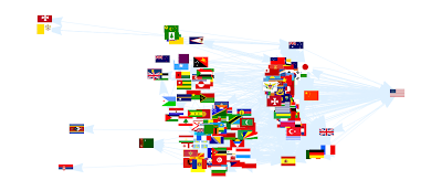
See the original.
VertexRenderingFunction -> (Inset[Show[CountryData[#2, "Flag"], ImageSize -> 30], #] &)

See the original.
Dec 27, 2007
Working with image: Mosaic images
Creating the image mosaic can be very easy in Mathematica.
First, what's inside the image?
Import["mnt.png", "Elements"]]
{"BitDepth", "ColorMap", "ColorSpace", "Data", "DataType", "Graphics", "GrayLevels", "ImageSize", "RawData", "RGBColorArray"}
We only need use the "Data": Import["mt.png","Data"]
Here we "steal" some images from Almighty Google as the example.
Import the following four images (a0,a1,a2,a3)
a0: http://mt0.google.com/mt?n=404&v=ap.66&x=0&y=0&zoom=16
a1: http://mt1.google.com/mt?n=404&v=ap.66&x=1&y=0&zoom=16
a2: http://mt1.google.com/mt?n=404&v=ap.66&x=0&y=1&zoom=16
a3: http://mt3.google.com/mt?n=404&v=ap.66&x=1&y=1&zoom=16
See these two guides for details on Quadtree coordinate system used by Google.
Coordinate systems for Google Maps and Google Satellite Images
Then create the data matrix for the new image:
mosaicimg=ArrayFlatten[{{a0, a1}, {a2, a3}}];
Draw the new image and export it:
Graphics[Raster[Reverse[mosaicimg]/255, ColorFunction -> RGBColor],
PlotRange -> {{0, 511}, {0, 511}}, ImageSize -> {512, 512}]
Export["earth.png",%,"PNG"]
This is the image used in Fun with image overlay: Google Map
Leader of the World?
Dec 26, 2007
Fun with image overlay: Google map
Here is another example on image overlay. This time, the image from Google map is used as reference image.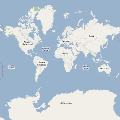
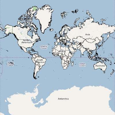
The image overlay is perfect! The secret is that the projection has to be matched. Google map currently uses Mercator projection.
CountryData["World", {"FullPolygon", "Mercator"}] will produce the map with Mercator projection.


The image overlay is perfect! The secret is that the projection has to be matched. Google map currently uses Mercator projection.
CountryData["World", {"FullPolygon", "Mercator"}] will produce the map with Mercator projection.
Fun with image overlay
Here shows the example to creating new maps in Mathematica by using image overlay.
Download the earthmap image
(*import reference image*)
refimage=Import["earthmap.png"];
(*create the overlay for earthmap image*)
overlayimage = Rasterize[
Graphics[Translate[{EdgeForm[Black], FaceForm[],
CountryData["World", "FullPolygon"]}, {180, 90}],
PlotRange -> {{0, 360}, {0, 180}}], ImageSize -> 1024,
Background -> None]
(*show two images together*)
Show[refimage,overlayimage]
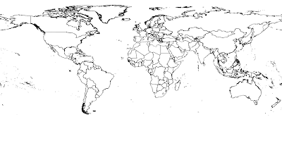
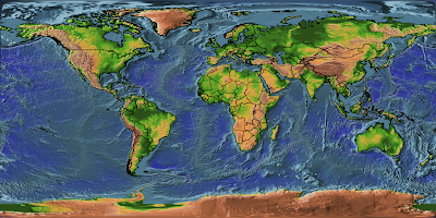
Several parameters are important here:
Translate[...,{180,90}]: the lower left corner of the reference image is always (0,0), the overlay image has to be moved to the same origin.
Background -> None: set overlay image with transparent background
ImageSize -> 1024: math the size of reference image
Download the earthmap image
(*import reference image*)
refimage=Import["earthmap.png"];
(*create the overlay for earthmap image*)
overlayimage = Rasterize[
Graphics[Translate[{EdgeForm[Black], FaceForm[],
CountryData["World", "FullPolygon"]}, {180, 90}],
PlotRange -> {{0, 360}, {0, 180}}], ImageSize -> 1024,
Background -> None]
(*show two images together*)
Show[refimage,overlayimage]


Several parameters are important here:
Translate[...,{180,90}]: the lower left corner of the reference image is always (0,0), the overlay image has to be moved to the same origin.
Background -> None: set overlay image with transparent background
ImageSize -> 1024: math the size of reference image
Dec 22, 2007
Improve mapping by importing new data
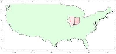
Compared to Matlab’s Mapping Toolbox, the mapping ability of Mathematica is rather rudimentary. The overall quality of built-in maps is poor and lack of details. The most annoying problem is that it can't import ESRI shapefile directly. Here is one simple example to show how you can import your own data. Boundaries of Indiana and Illinois in shapefile format are exported to csv format (x,y), then import csv file and display as Polygon. The imported data works well with the built-in map.


Dec 21, 2007
Playing with numbers: Oil Consumption
Ok, everyone knows the fact:
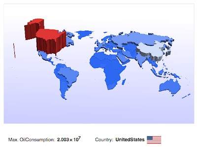 (It's probably the data of year 2005)
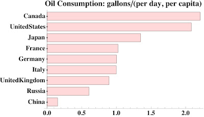
oil consumption in barrels per day
 (It's probably the data of year 2005)
G8 vs China

Dec 20, 2007
Common city names shared between USA and Mexico
m = Take[First /@ CityData[{All, #}]] & /@ {"UnitedStates", "Mexico"};
cityname = Intersection[m[[1]], m[[2]]]
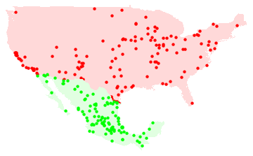
{"AguaDulce", "Alamo", "Algodones", "Alvarado", "Anahuac", "Belen", "Camargo", "Carbon", "Carmen", "Cerritos", "CerroGordo", "Chalco", "China", "Colon", "Concordia", "Delta", "Duarte", "Durango", "Eldorado", "ElRefugio", "Gonzalez", "Guadalupe", "Hercules", "Hidalgo", "LaJoya", "LaPalma", "LaPaz", "LaPresa", "Leon", "LosAltos", "Madera", "Madrid", "Magdalena", "Martinez", "Medina", "Mina", "Miramar", "Naco", "Nogales", "Oriental", "PaloAlto", "Progreso", "RioBravo", "RioGrande", "Rodeo", "Salamanca", "Salinas", "Saltillo", "SanBernardino", "SanBuenaventura", "SanCarlos", "SanFelipe", "SanFernando", "SanGabriel", "SanIgnacio", "SanLucas", "SanLuis", "SanMarcos", "SanPatricio", "SanPedro", "SanRafael", "SantaAna", "SantaBarbara", "SantaClara", "SantaTeresa", "Soledad", "Sonoita", "Tampico", "Toluca", "Torreon", "Valparaiso", "Victoria"}
cityname = Intersection[m[[1]], m[[2]]]

{"AguaDulce", "Alamo", "Algodones", "Alvarado", "Anahuac", "Belen", "Camargo", "Carbon", "Carmen", "Cerritos", "CerroGordo", "Chalco", "China", "Colon", "Concordia", "Delta", "Duarte", "Durango", "Eldorado", "ElRefugio", "Gonzalez", "Guadalupe", "Hercules", "Hidalgo", "LaJoya", "LaPalma", "LaPaz", "LaPresa", "Leon", "LosAltos", "Madera", "Madrid", "Magdalena", "Martinez", "Medina", "Mina", "Miramar", "Naco", "Nogales", "Oriental", "PaloAlto", "Progreso", "RioBravo", "RioGrande", "Rodeo", "Salamanca", "Salinas", "Saltillo", "SanBernardino", "SanBuenaventura", "SanCarlos", "SanFelipe", "SanFernando", "SanGabriel", "SanIgnacio", "SanLucas", "SanLuis", "SanMarcos", "SanPatricio", "SanPedro", "SanRafael", "SantaAna", "SantaBarbara", "SantaClara", "SantaTeresa", "Soledad", "Sonoita", "Tampico", "Toluca", "Torreon", "Valparaiso", "Victoria"}
Dec 19, 2007
Top 10 most common city names in USA
(*Total 28184 USA city names *)
Take[SortBy[Tally[First /@ CityData[{All, "UnitedStates"}]], Last], -10]
{{"Fairview", 21}, {"Georgetown", 21}, {"Marion", 21}, {"Greenville", 23}, {"Madison", 23}, {"Salem", 24}, {"Springfield", 24}, {"Washington", 25}, {"Clinton", 26}, {"Franklin", 28}}
Where are the "Clinton"?
Graphics[{LightBlue, CountryData["UnitedStates", "Polygon"],
PointSize[Medium], Red,
Point[Reverse[CityData[#, "Coordinates"]]] & /@
CityData[{"Clinton", "UnitedStates"}]}]
Subscribe to:
Comments (Atom)


