Geospatial function: Point in Ploygon Test

There is an excellent post on point in polygon test from Mathematica Stackexchange.

Point in polygon test is one of the most useful functions when processing Geospatial data. Unfortunately, there is no official built-in function from Mathematica yet. Here is an example of showing usefulness of this function.
We have some data on Greenland icesheet thickness in format of {lon,lat, thickness}.

Our goal is to make a map to show the thickness of icesheet.
First try with ListDensityPlot:

You can see it is not working well, we need to limit the plot region inside the boundary of Greenland. Here is the place we can use the point-in-polygon test. In this example, I use inPolyQ2 from the answer by Simon Woods:

Still not right? What's wrong? The trick is to increase MaxPlotPoints  to 100 at least:

ListDensityPlot[data, PlotRange -> All,
 ColorFunction -> (ColorData["Rainbow"][1 - #] &),
 RegionFunction -> (inPolyQ2[greenland_ploygon[[1, 1]], #1, #2] &),
 MaxPlotPoints -> 150, MeshFunctions -> {#3 &}, Mesh -> 10]

It looks like a real map now.

Fetching data from HTML source

Parsing html to get the data we need can be very frustrating. Lucky, Mathematica has a powerful hmtl import function, you can import raw html data into several different formats. In my experiences, import html as "XMLObject" is usually the best way to go. 
Here is an example: OSCAR Nominees:

xml = Import["http://oscar.go.com/nominees", "XMLObject"];   

We are interested in the list of nomineed films

body = Cases[xml, XMLElement["div", {"class" -> "nominee-by-film"}, ___], Infinity];

Extract titles:

title = Cases[body, XMLElement["span", {"class" -> "title"}, value_] :> value, Infinity] 

Extract the number of nominees:

nominee =
  Cases[body,
   XMLElement["h1", {"class" -> "numberOfNominations"}, value_] :>
    StringCases[value, x : NumberString :> ToExpression[x]], Infinity] ;

Put these two together:

result = Sort[Transpose[{title, Flatten@nominee}], #1[[2]] > #2[[2]] &]

Let's draw a graph to show the top 10 of the most nomineed films:

oscar = Import["http://www.oscars.org/awards/academyawards/about/awards/images/side_oscar.jpg"];
BarChart[result[[1 ;; 10, 2]],
 ChartLabels -> Placed[Flatten@result[[1 ;; 10, 1]], After],
 BarOrigin -> Left, Background -> LightBlue, ChartElements -> {oscar, {1, 1}},
  Axes -> None, LabelStyle -> {Bold, Darker@Blue, 14}] 

For this particular example, you can also try to get the same information directly from WolframAlpha.

Related post: A discussion on Mathmeatica Stackexchange

Simple Guide on Geospatial Coordinates Transformation with Mathematica

A few questions on geospatial coordinates transformation have shown up in Mathematica.Stackexchange. Here is a very brief summary.

In US, you probably likely deal with two projection systems: State Plane Coordinates System and UTM.

1. State Plane Coordinates System
In the U.S. State Plane Coordinate System (SPCS), the transverse Mercator projection is used for states that are long in the north-south direction, a Lambert conformal conic projection is used for states that extend in the east-west direction, and the oblique Mercator projection is used for Alaska.

In GeoProjectionData, SPCS83IN01 and SPCS83IN02 represent Indiana Steate Plane east zone and west zone. SPCS83TX01 ~ SPCS83TX05 represent 5 zones from north to south in Texas. Tennessee has only one zone: SPCS83TN00. Here is an online interactive map on SPCS.

There are also SPCS27 series, which are based on NAD27 datum, however, it is quite rare to get the data in the old coordinate system.

One common mistakes is usually caused by the unit: meters vs feet. In Mathematica, the coordinate is calculated in meters, the data you get is probably in feet.

Related posts on stack exchange convert spcs to (lat, lon), convert (lat, lon) to spcs

2. UTM
Universal Transverse Mercator (UTM) coordinate system divides the Earth into sixty zones: UTMZone01 ~ UTMZone60.

In Mathematica 9, there is a problem with UTMZone data:

GeoProjectionData["UTMZone16"]
{"TransverseMercator", {"Centering" -> {0, -87},  "CentralScaleFactor" -> 1, "GridOrigin" -> {0, 0}, "ReferenceModel" -> "WGS84"}}

The scale factor: 0.9996 and the grid origin: {500000,0} shall be specified for coordinate transformation: 

GeoGridPosition[
 GeoPosition[{39.162147, -86.529045}, "WGS84"], {"UTMZone33",
  "CentralScaleFactor" -> 0.9996, "GridOrigin" -> {500000, 0}}]

Related posts on stack exchange convert between (lat, lon) and UTM

This problem is fixed in next version of Mathematica.

Testing Wolfram Language on a Raspberry Pi emulation

Want to test Wolfram Language without a Raspberry Pi? 

Files you need to download for Windows platform:

1. QEMU 1.6.0 Binary for Windows: Qemu-1.6.0-windows.zip
2. Linux Kernel
3. Latest Raspbian Image 2013-09-25-wheezy-raspbian.zip as this blog is written
4. The guide on Howto setup Raspberry Pi Emulation with Qemu on Linux or Windows

Main steps:

   1. expand Raspbian image to add more disk space

   2. start the virtual machine to register extra disk space

   3. install Mathematica Language:

       sudo apt-get update && sudo apt-get install wolfram-engine

   

Once you get it running, you can check the performance against a real Raspberry Pi

It takes around 1 hour to get it done. Don't expect much on the performance, have fun!

Updates:

Remote Development Kit doesn't work, the reason is "ssh"

To ssh into the emulated Raspberry Pi, add "-redir tcp:2222::22" to the command options when starting qemu, then "ssh -p 2222 pi@localhost", in Mathematica, it probably connects port 22 by default, it seems no way to specify the port number.

How to make arrow objects for Google Earth

In the previous post, we has use GeoDestination function to make circle objects, and we can use the same function to generate arrow objects, too.

The data we have is the position and displacements in north and east direction, {lat, lon, ndis, edis}. ndis, edis is in millimeter in this case.

First, let calculator the length of the arrow, the scale here is 1 mm displacement = 1000 meters

length = Sqrt[ndis^2 + edis^2]*1000

Then the angle. GeoDestionation requires GeoDirection, it starts from the north.

angle = ArcTan[edis, ndis] /Degree
geoangle = 90 - angle

For the end point:

end = First@GeoDestination[{lat, lon}, {length, geoangle}]

The trick to generate the arrow is that to form another smaller circle around the end point, pick up two points from the arrow heads. 

arr1 = First@GeoDestination[end, {dist*.25, geoangle + 180 - 30}]
arr2 = First@GeoDestination[end, {dist*.25, geoangle - 180 + 30}]

Then we can have two lines which draw in this order, {org –> end}, {arr1->end->arr2}. When comes to export kml, we need to use <MultiGeometry> object in KML, it seems not supported by Export function in Mathematica yet, so you can just export the following string directly:

<MultiGeometry>
<LineString>
<tessellate>1</tessellate>
<coordinates>
-117.093195026,34.116408002,0 -117.020521006,34.0741018797,0
</coordinates>
</LineString>
<LineString>
<tessellate>1</tessellate>
<coordinates>
-117.042636322,34.0757361767,0 -117.020521006,34.0741018797,0 -117.029869517, 34.0907835742, 0
</coordinates>
</LineString>
</MultiGeometry>

Here is the screenshot of the final product in Google Earth:

How to make a circle for Google Earth

KML doesn’t have the circle object built in, a circle can be made by line or polygon object. With GeoDestination function, a perfect circle can be created.

Polygon@Table[GeoDestination[GeoPosition[{39.17, -86.52 }], {5000, a}], {a, 0, 360, 10}][[All, 1, {2, 1}]]

This line will generate a 36-sides polygon centered at 39.17, –86.52 with 5000 meters radius. Then export it to kml, you probably has to manually modify the kml file to set up the color styles.

Here is an example, we use the radius to represent the vertical motion, 1 cm motion = 5000 meters on the ground.

Mathematica and Spatial Database

Warning: this post uses undocumented Mathematica command and modifies the Mathematica installation. Don't try this at home.

For any GIS software, evaluating spatial relationships, such as equal, disjoint, within, intersects, etc., is a fundamental requirement. Also, R-tree support is a must for any large spatial data set. Currently, these sets of functions are not built in Mathematica. It is difficult to perform complex GIS analysis inside Mathematica. One way is to call external libraries through Mathlink/Jlink. Another way is connecting to a spatial database, such as PostGreSQL, Oracle Spatial through database connection. Spatial database? What about Spatialite, it is a complete spatail DBMS built as an extension to the extreme light-weighted database SQLite. 

From this Wolfram|Alpha tweet analysis post, it shows Mathematica actually ship with SQlite.

I installed the Mathematica 8 linux trail version.

db = Database`OpenDatabase["/tmp/test.sqlite"];
Database`QueryDatabase[db, "SELECT sqlite_version();"]
{{3.6.1}}

Here is SQLite library from Mathematica
/usr/local/Wolfram/Mathematica/8.0/SystemFiles/Kernel/Binaries/Linux/libsqlite3.so

For security reason, the dynamic loading extension is disabled. And we need to compile our own copy of libsqlite3.so. The detail is explained here: the pre-packaged 'libsqlite' trap.

Grab the source code for SQLite website, build the new library with:

CFLAGS="-DSQLITE_ENABLE_LOAD_EXTENSION=1" ./configure

then make a copy of the original libsqlite3.so, and overwrite it with the new version.

Database`QueryDatabase[db, "SELECT sqlite_version();"]
{{3.7.5}}

Then we can try with the Spatialite already installed:

Database`QueryDatabase[db, "SELECT load_extension(‘/usr/lib/libspatialite.so’);"]
Database`QueryDatabase[db, "SELECT spatialite_version();"]
{{"2.4.0"}}

Try a spatial SQL command:

Database`QueryDatabase[db, "SELECT X(GeomFromText('POINT(-85 39)',4326));"]
{{-85.}}

Wow, it is working!

Here is a tutorial on Spatialite, you can get the idea of what kind of functions are supported by Spatialite. If you are familiar with the spatial database, you can build a rather functional GIS system inside Mathematica with the support of Spatialite.

Create simple DEM from Google Map

With texture support in Mathematica 8.0, we can create the simple DEM with image overlay by combing the functions from two previous posts Google Static Map and Google Elevation API.

 

However, there is the usage limits on Google Elevation API. You’d better pull the dem once and export the data, otherwise, you may hit the daily limits very quickly.

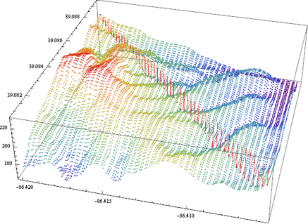
Here is an example on displaying earthquake data with the dem, the red line outlines the fault plane.

Download notebook.

Color-coded contour lines with Mathematica

In ContourPlot, ContourStyle –> function can be used to color-code contour lines.For example, the number of contours is numC=20, then for each contour, the color is defined by a coloring function:

ContourStyle -> Table[{ColorData["Rainbow", (i - 1)/(numC - 1)]}, {i, numC}]

Of course, it is also necessary to set Contours –> numC.

Here are the examples, the famous peaks function from Matlab is used.

2D ContourPlot example:

Turn 2D plot into the 3D one:

Another 3D example:

Download the notebook.

Customizing DateListPlot with PlotMarkers

This example shows you how to specific PlotMarkers for each point in a data set. The solution is quite simple, just partition the dataset into different series, each set only contains one point exactly: Partition[data, 1]. Then we can assign the different PlotMarkers for each point.

Let’s download some weather data:

data = WeatherData[$GeoLocation, "WindDirection", {{2009, 1, 1}, {2009, 1, 5}}];
data = Select[data, FreeQ[#, {_, Missing["NotAvailable"]}] &];

We like to use arrows to represent wind directions:

markers =
  Graphics[{Red, Arrow[{{0, 0}, -0.5 {Sin[#[[2]] Degree], Cos[#[[2]] Degree]}}],
      EdgeForm[], FaceForm[], Rectangle[{-1, -1}, {1, 1}]}] & /@ data;

We put a invisible box around arrow to make sure that the markers are aligned by {0, 0}.

newdata = data; newdata[[All, 2]] = 0;
g = DateListPlot[Partition[newdata, 1], PlotRange -> All, PlotMarkers -> markers, Axes -> {True, False}, FrameTicks -> {Automatic, None}]

Let’s test another place: Tokyo, Japan

Summer time:

 

Winter time:

The pattern of winter “north” wind and the summer “south” wind is very clear, it is much better than just plotting points.

No notebook, all the codes are here already.

Plotting on Google static map

We have given an example on plotting with WMS. You may be wondering how we can do the similar thing with Google static map. It is very easy to use with Mathematica:

googleMap[{lat_,lon_},{sizex_,sizey_},zoom_,maptype_]:=Import["http://maps.google.com/maps/api/staticmap?sensor=false&center="<>ToString[lat]<>","<>ToString[lon]<>"&zoom="<>ToString[zoom]<>"&size="<>ToString[sizex]<>"x"<>ToString[sizey]<>"&maptype="<>maptype];

Google map is based on Mercator Projection. So the data has to be projected, rather than drawing (longitude, latitude) pairs directly. The scale on east-west (longitude) is constant with zoom level, and only latitude needs to be projected.

(* convert lat to y *)
lat2y[lat_]:=0.5Log[(1+Sin[lat Degree])/(1-Sin[lat Degree])];
(* convert y to lat *)
y2lat[y_]:=Gudermannian[y]*180/Pi;

We have the data in pairs of (longitude, latitude) which lie in a bounding box ((lon1,lat1), (lon2, lat2)), and to plot them on a Google static map, we need: 1. find the center of the map; 2. find the right zoom level; 3. find the proper map size; 4. project the data: (longitude, lat2y[latitude])

I will skip the details, if you are interested into the mathematics, check out these two posts, : R-Google Map and How to make Google static maps interactive.

Here are two examples:

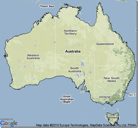
coords = CountryData["Australia", "Coordinates"];
(* only project latitude *)
Map[{#[[2]],lat2y[#[[1]]]}&, coords,{2}]]

In the second example, GIS data is imported from an XML file, it is from the post before Mathematica 7.0 released.

Mathematica 8 has the texture function, so we can import static Google map as the texture, it will be easy to create complex 3D GIS visualization.

Download the notebook for detail.

Extract elevation data with Google Elevation Service

In the previous post: Extract elevation data from Google Earth, Google Earth COM API is used, it only works on Windows platform. Google Map now has Elevation Web Service, it is quite easy to do it with new API. The new service does not require a Maps API key. The basic form is

“http://maps.google.com/maps/api/elevation/outputFormat?parameters”

For output format, 

• /json returns results in JavaScript Object Notation (JSON).
• /xml returns results in XML, wrapped within a <ElevationResponse> node.

JSON is easy to parse, this is a sample query:
json=Import["http://maps.google.com/maps/api/elevation/json?locations=39.7391536,-104.9847034&sensor=false"]

{
  "status": "OK",
  "results": [ {
    "location": {
      "lat": 39.7391536,
      "lng": -104.9847034
    },
    "elevation": 1608.8402100
  } ]
}

ToExpression@StringCases[json, NumberString]

{39.7392,-104.985,1608.84}

Here is the example output:

Path elevation example:

DEM + Path:

Grab the GoogleElevationService.nb for detail.

Update: answer the comments

You may have the trouble with the notebook. Sometimes ListPlot3D runs too slow and even crashes Mathematica. You can switch to ListPlotPoint3D.

ListPointPlot3D[dem[[All, {2, 1, 3}]], ColorFunction -> "Rainbow"]

Here is the example with 100 by 100 DEM.

More on Heatmap

A reader asks about this heatmap post on Flowing Data. Sure, we can do it easily with ArrayPlot. Grab the notebook here.

data = Import["ppg2008.csv"];

Grid[data]

 

numbers = data[[2 ;; All, 2 ;; All]]; (* this is the data for heatmap *)
playernames = data[[2 ;; All, 1]]; (* for the labels *)
statnames = data[[1, 2 ;; All]]; (* for the labels *)

Then we need to scale the each column separately to [0,1].

newnumber = Transpose[Rescale[#] & /@ (Transpose[numbers])];

Then you can generate a simple heatmap simply by ArrayPlot[newnumber].

Of course, we like to add the labels with FrameTicks option. FrameTicks->{{left,right},{bottom,top}}  mark options specified separately for each edge. 

Transpose[{Range[Length[playernames]], playernames}] generate the list {{1, “player1”} … {50, “player50”}} to label the player names.

Transpose[{Range[Length[statnames]], Map[Rotate[#, 60 Degree] &, statnames]}] with this line, we can rotate the labels at the same time.

Here is the final product, click to see the full graphic.

Charting time series as calendar heat maps

I haven’t updated this blog for a while. I am working on one Matlab project right now. It is kind of difficult for me to work with Matlab and Mathematica at the same time.

There is an interesting post Charting time series as calendar heat maps in R. The original idea from SAS Analysis of airline performance. I create a simple version in Mathematica. The tricky part is to generate the background grid.

The code I use is from an old tutorial of Making a Calendar. For each month, the boundary is defined by 8 points, marked out by darker line. The monthly grids are shifted to the right positions to form a yearly grid. Once you figure out this part, the rest is just straightforward.

I use the stock as the example, this  is actually not the best data set for this type of visualization.

Calendar heatmap:

Download the file calendarheatmap.nb for the detail.

By the way, you can do whatever you like with the materials posted on this blog, there is no copyright problem.

User-defined color themes

With Blend function, it is quite simple to use user-defined color themes.

Blend[{col₁, col₂, col₃, ...}, x]: linearly interpolates between colors col_i as x varies from 0 to 1.

We like to use the following color theme:

c = {{37, 57, 175}, {40, 127, 251}, {50, 190, 255}, {106, 235,
    255}, {138, 236, 174}, {205, 255, 162}, {240, 236, 121}, {255,
    189, 87}, {255, 161, 68}, {255, 186, 133}, {255, 255, 255}};

colors = RGBColor[#/255] & /@ c;

This shows the each color in the theme:

Graphics[Table[{EdgeForm[Black], FaceForm[colors[[i]]],
   Rectangle[{i, 0}, {i + 1, 1}]}, {i, 1, Length[colors]}]]

Check the color theme with Blend function:

DensityPlot[x, {x, 0, Length[c]}, {y, 0, 1}, AspectRatio -> Automatic,
  FrameTicks -> None, ColorFunction -> (Blend[colors, #] &),
PlotRangePadding -> None]

Then you probably notice how to use it in your own plot,

ColorFunction -> (Blend[colors, #] &)

Test the color theme with the data:

ReliefPlot[data, ColorFunction -> (Blend[colors, #] &)]

Maybe the ligher color is better.

lightercolors = Lighter[#] & /@ colors;

Just for fun, let’s play the color theme with an existing image.

img=ImageData[ColorConvert[place_any_image_here, ”Grayscale”]];

ArrayPlot[img, ColorFunction -> (Blend[darkercolors, #] &)]

Wikipedia Page Analysis

Wikipedia has lots of scientific information, however, due to its nature, it is still not considered as a research resource.  This doesn’t mean it has to be ignored. I have checked some pages related with various topics in GIS field. Most of them are well-written, the information are actually quite accurate, several contributors are the professionals in the field. In this post, I like to check some metadata information of  “Mathematica” Page on Wikipedia, it may gives us some ideas about its quality.

Tools we need: Mediawiki API and Mathematica. There are plenty examples on how to use Mediawiki api. Basic procedure is to use Import[queryurl,”XML”], then parse xml to get the information we need.

Page revision history:

(* import  contributor and timestamp *)

url = "http://en.wikipedia.org/w/api.php?action=query&prop=revisions&\
titles=Mathematica&rvprop=user|timestamp&rvlimit=500&redirects$rvuser&\
format=xml";

xml = Import[url, "XML"];
rawdata= Cases[xml, XMLElement["rev", w_, _] :> w, Infinity];
data = {"user", "timestamp"} /. rawdata;

 

 

This page is constantly revised, we probably can assume the information on “Mathematica” page is up-to-date.

The information on the contributors is also interesting.

 

We can dig out more information on the contributors:

(* import paged edited by each user *)

userpages[usr_] :=
  Module[{url, uxml, udata, unicase},
   url = "http://en.wikipedia.org/w/api.php?action=query&list=\
usercontribs&uclimit=500&format=xml&ucuser=" <> usr;
   uxml = Import[url, "XML"];
   udata = Cases[uxml, XMLElement["item", w_, _] :> w, Infinity];
   unicase = DeleteCases[Union["title" /. udata ],
     x_ /; (StringMatchQ[x, "User talk:" ~~ __] || StringMatchQ[x, "Talk:" ~~ __] || StringMatchQ[x, "User:" ~~ __])]; Map[usr -> # &, unicase]];

 

The common pages edited by these top5 contributors:

  

From the pages they have edited, they have worked on several topics closely related with Mathematica. This looks good, we may say they probably know what they are doing.

Update:

Download Wikipedia Notebook for the details.

View weighted graph with GraphPlot

Here is a simple example on how to customizing Graphplot. We like to use GraphPlot to visualize the number of people who commute into or out Monroe county from/to its neighbor counties.

g={{"Owen" -> "Monroe", 2813}, {"Greene" -> "Monroe",
  3788}, {"Lawrence" -> "Monroe", 4022}, {"Jackson" -> "Monroe",
  85}, {"Brown" -> "Monroe", 689}, {"Morgan" -> "Monroe",
  821}, {"Monroe" -> "Owen", 676}, {"Monroe" -> "Greene",
  207}, {"Monroe" -> "Lawrence", 679}, {"Monroe" -> "Brown",
  303}, {"Monroe" -> "Morgan", 617}}

vercoor={"Monroe" -> {-86.529, 39.1621}, "Owen" -> {-86.7642, 39.2868}, "Greene" -> {-86.9403, 39.0246},  "Lawrence" –> {  -86.4923,  38.8627}, "Jackson" -> {-86.0462, 38.8798},  "Brown" -> {-86.2382, 39.203}, "Morgan" -> {-86.4238, 39.4233}}

First try:

GraphPlot[g, VertexLabeling -> True, VertexCoordinateRules -> vercoor]

Using arrow to indicate in/out seems to be a good idea. We use EdgeRenderingFunction in second try:

GraphPlot[g, VertexLabeling -> True,
EdgeRenderingFunction -> (Arrow[#1, 0.05] &),
VertexCoordinateRules -> vercoor]

However, the labels on the edge is lost. We can handle it in EdgeRenderingFunction.

GraphPlot[g, VertexLabeling -> True,
EdgeRenderingFunction -> ({Text[#3, Mean[#1]], Arrow[#1, 0.05]} &),  VertexCoordinateRules -> vercoor]

The graph is still difficult to read, the commuting pattern isn’t clear at a glance. We further update EdgeRenderingFunction and use the line color and thickness to show the pattern.

GraphPlot[g,
EdgeRenderingFunction -> ({If[#2[[1]] == "Monroe", Red, Blue],
     AbsoluteThickness[0.5 + #3/500], Arrowheads[0.02 + #3/120000],  Arrow[#1, 0.05]} &), VertexLabeling -> True,
VertexCoordinateRules -> vercoor]

In the last try, we use VertexRenderingFunction to make the label more clear.

GraphPlot[g,
EdgeRenderingFunction -> ({If[#2[[1]] == "Monroe", Red, Blue],
     AbsoluteThickness[0.5 + #3/500], Arrowheads[0.02 + #3/120000], Arrow[#1, 0.06]} &), VertexLabeling -> True,
VertexCoordinateRules -> vercoor,
VertexRenderingFunction -> ({Text[Style[#2, 14, Bold], #2 /. vercoor, Background -> White]} &)]

Import the shapefile, then you get a map:

Extract elevation data from Google Earth

In Google Earth COM API, there is a function: GetPointOnTerrainFromScreenCoords

Given an screen_x and screen_y, it returns IPointOnTerrainGE object, which gives out the {Latitude, Longitude, Altitude}

Screen coordinates range from (-1, –1) to (+1, +1)

(-1, -1) - bottom left hand corner of the screen. (0,0) - center of the screen. (1, 1) - top right hand corner of the screen.

Let’s use this function in Mathematica to extract elevation data.

First, zoom Google Earth into a testing place

Then in Mathematica:

Needs["NETLink`"]
InstallNet[]
ge = CreateCOMObject["GoogleEarth.ApplicationGE"];

getAltitude[x_, y_] :=
  Module[{pv},
   pv = ge@GetPointOnTerrainFromScreenCoords[x, y]; {pv@Longitude, pv@Latitude, pv@Altitude}];

(* extract 50 by 50 grids around the center of the screen *)
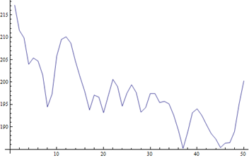
dem = Table[
   getAltitude[x, y], {x, -0.5, 0.5, 0.02}, {y, -0.5, 0.5, 0.02}];

 

 

Next situation: Given a list of {Latitude, Longitude}, how can we get the corresponding elevations for each location?

The tip is to use the camera control to move the center of screen to the given  {Latitude, Longitude}.

cam = ge@GetCamera[1];

getAltitudebyLatLon[{lat_, Lon_}] :=
Module[{pv}, cam@FocusPointLongitude = Lon;
  cam@FocusPointLatitude = lat; cam@Range = 8000; ge@SetCamera[cam, 5];
  pv = ge@GetPointOnTerrainFromScreenCoords[0, 0]; pv@Altitude]

cam@Range is the control of “eye alt”, it is in meters.

It comes very handy for extracting the cross-profile.

Control Google Earth from Mathematica

This is for Windows platform only. With Mathematica’s .NET link and Google Earth COM API, we can control Google Earth’s camera and add features directly from Matheamtica.

There is an example of planning a shortest tour through every country of the world in Document: FindShortestTour.

SC[{lat_,lon_}]:=r {Cos[lon \[Degree]] Cos[lat \[Degree]],Sin[lon \[Degree]] Cos[lat \[Degree]],Sin[lat \[Degree]]};
r=6378.7;
places=CountryData["Countries"];
centers=Map[CountryData[#,"CenterCoordinates"]&,places];
distfun[{lat1_,lon1_},{lat2_,lon2_}]:=VectorAngle[SC[{lat1,lon1}],SC[{lat2,lon2}]] r;
{dist,route}=FindShortestTour[centers,DistanceFunction->distfun];

Let’s view this example in Google Earth:

Needs["NETLink`"]
InstallNET[];

(* startup google earth *)
ge = CreateCOMObject["GoogleEarth.ApplicationGE"];

(* load path file already generated *)
ge@OpenKmlFile["d:/temp/test2.kml",1]

(* get the camera object *)
cam=ge@GetCamera[1];

(* funcion to ratate the camera *)
runcam[{lat_,lon_}]:=Module[{},
cam@FocusPointLongitude=lon;
cam@FocusPointLatitude=lat;
ge@SetCamera[cam,2]];

(* let's see the movie *)
runcam[#]&/@ centers[[route]];

Here is a low quality video.

 

Here is test2.kml for the shortest path

Here is the recorded tour (shortestrout.kmz) in Google Earth

First load test2.kml to Google Earth, then double click ShortestRoute.kmz to view the animation.

Mathematica 7: Export ESRI shapefile

One way to achieve this goal is by using the spatial database. Oracle and PostgreSQL have excellent supports of spatial data types. All you need to do is to connect the database in Mathematica and insert the data into the spatial database. There are tools come with databases allow you to dump the data into a shapefile. If you need a light-weighted spatial database, you can try SpatiaLite, it is based on popular SQLite.

For Windows platform, download the followings first:

spatialite-tools and init_spatialite-2.3.sql

upzip them and copy spatialite.exe and init_spatialite-2.3.sql into the same folder.

In this example, we like to export the following information to a shape file:

data={First[#], CityData[#,"Population"], CityData[#,"Longitude"], CityData[#,"Latitude"]} &/@ CityData [{All, "Indiana", "UnitedStates"}];

We need write some SQLs:

CREATE TABLE Towns (Name TEXT, Population INTEGER);
SELECT AddGeometryColumn('Towns','LonLat', 4326,'Point',2);

4326 means  EPSG 4326, the coordinate reference system of WGS84(longitude, latitude) pair coordinates in degrees.

To Insert the data:

INSERT INTO Towns (Name, Population, LonLat) Values ('Indianapolis', 784118, GeomFromText ('Point(-86.1477 39.7909)', 4326));

In Mathematica, this will create all the “INSERT” statements

str="INSERT INTO Towns (Name, Population, LonLat) Values ('v1', v2, GeomFromText('Point(v3 v4)',4326));"

strs=StringReplace[str, {"v1"->#[[1]], "v2"->ToString[#[[2]]],"v3"->ToString[#[[3]]], "v4"->ToString[#[[4]]]}] &/@ data;

Export["insert.txt", strs]

Then we can put all the SQL statements together into one file (test.sql):

BEGIN;
CREATE TABLE Towns (Name TEXT, Population INTEGER);
SELECT AddGeometryColumn('Towns','LonLat', 4326,'Point',2);
… INSERT INTO commands is here …
COMMIT;

In window command line mode:

spatialite.exe -init init_spatialite-2.3.sql test.sqlite < test.sql

So far, we have got all the data from Mathematica into the table Towns in test.sqlite.

run: spatialite.exe test.sqlite, and check if the records inside are right, then dump the shapefile:

.dump Towns LonLat towns_shp ASCII POINT;

Import the town_shp.shp back into Mathametica:

Show[Import["towns_shp.shp"], Frame -> True, FrameTicks -> Automatic]

More information: SpatiaLite Tutorial

If you are not comfortable with command-line tools, there is a GUI tool for SpatiaLite.